
A Machine Learning-Based Approximation of Strong Branching
論文閱讀筆記,個人理解,如有錯誤請指正,感激不盡!該文分類到Machine learning alongside optimization algorithms。
01 Introduction
目前大部分 mixed-integer programming (MIP) solvers 都是基于 branch-and-bound (B&B) 算法。近幾年很多新的特性如cutting planes, presolve, heuristics, and advanced branching strategie等都被添加到了MIP solvers上以提高求解的效率。
branching strategie對MIP的求解效果有著很大的影響,也有很多文獻(xiàn)對其進(jìn)行了研究。
最簡單的branching strategie為 most-infeasible branching,即每次選擇小數(shù)部分最接近0.5的變量進(jìn)行分支。還有 pseudocost branching,該策略首先對分支過程中的dual bound increases進(jìn)行一個記錄,然后在分支的時候利用該信息對候選變量的dual bound increases進(jìn)行一個評估,這種方法有個缺點就是一開始的時候沒有足夠的信息可供使用。strong branching則克服了這一缺點,它通過計算每個fractional variable分支后的linear programming (LP) relaxations,從而顯式地評估dual bound increases,然后最大的 increases就作為當(dāng)前分支的節(jié)點。它的效果是顯而易見的,但是,分支節(jié)點過多,每次求解LP relaxations需要花費(fèi)過多的時間,導(dǎo)致了strong branching的求解效率過低。當(dāng)然還有很多分支策略,例如 reliability branching,inference branching和nonchimerical branching等,感興趣的可以去讀讀文獻(xiàn)。
這篇文章的contribution在于,利用機(jī)器學(xué)習(xí)的方法,對strong branching進(jìn)行了學(xué)習(xí),并模型集成到B&B算法的框架中,以加速算法的求解速度。
這篇文章處理的二進(jìn)制MILP問題有如下的形式:
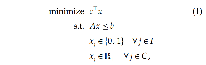
其中,分別表示成本系數(shù)和系數(shù)矩陣。在右邊,和分別為整數(shù)變量和實數(shù)變量的下標(biāo)集合。
02 Learning Branching Decisions
本文并不是提出一個新的branching heuristic,而是使用machine learning通過學(xué)習(xí)模仿其他分支策略生成的決策去構(gòu)建一個branching strategy。本文的目標(biāo)是創(chuàng)造一個效率更高的strong branching的approximation。
2.1 Data Set Generation
機(jī)器學(xué)習(xí)首先是收集數(shù)據(jù)對,其中為當(dāng)前分支節(jié)點中待分支變量的特征值,而則是該特征對應(yīng)的標(biāo)簽。對模型進(jìn)行訓(xùn)練。收集數(shù)據(jù)可以使用strong branching對training problems進(jìn)行求解,并將求解的中間過程記錄下來。具體就是每個節(jié)點分支變量的特征以及標(biāo)簽值,這些數(shù)據(jù)最終作為機(jī)器學(xué)習(xí)算法的輸入而對模型進(jìn)行訓(xùn)練。
2.2 Machine Learning Algorithm
在這篇文章中,使用的算法為Extremely Randomized Trees或者ExtraTrees。ExtraTrees是從隨機(jī)森林直接修改過來的,之所以選擇ExtraTrees是因為它對于參數(shù)的取值具有較強(qiáng)的robust性。
03 Features Describing the Current Subproblem
特征對于機(jī)器學(xué)習(xí)算法來說是非常重要的,他們對方法的有效性起著關(guān)鍵作用。一方面,特征需要足夠完整和精確以更加準(zhǔn)確地描述子問題。而另一方面,他們又需要在計算中足夠高效。這兩方面是需要權(quán)衡的,因為有一些特征對方法的效果起著非常顯著的作用,但是計算的代價又非常大。比如,在分支過程中,對某支進(jìn)行分支時LP目標(biāo)值的提升值,就是一個非常好的特征,也在strong branching中使用了。但是計算這個值需要消耗的代價還是太大了,因此不適合該文的算法。
至于要選擇哪些特征,又是處于什么樣的考慮,作者也說了很多。感興趣的可以看看論文。下面是詳細(xì)的特征介紹,比較重要,因此直接把原文搬過來了。
3.1 Static Problem Features
The first set of features are computed from the sole parameters and . They are calculated once and for all, and they represent the static state of the problem. Their goal is to give an overall description of the problem. Besides the sign of the element , we also use and . Distinguishing both is important, because the sign of the coefficient in the cost function is of utmost importance for evaluating the impact of a variable on the objective value. The second class of static features is meant to represent the influence of the coefficients of variable in the coefficient matrix . We develop three measures—namely, , and — that describe variable within the problem in terms of the constraint . Once the values of the measure are computed, the corresponding features added to the feature vector are given by and . The rationale behind this choice is that, when it comes to describing the constraints of a given problem, only the extreme values are relevant. The first measure is composed of two parts: computed by such that , and computed by such that . The minimum and maximum values of and are used as features, to indicate by how much a variable contributes to the constraint violations. Measure models the relationship between the cost of a variable and the coefficients of the same variable in the constraints. Similarly to the first measure, is split in with , and with . As for the previous measure, the feature vector contains both the minimum and the maximum values of and . Finally, the third measure represents the inter-variable relationships within the constraints. The measure is split into and . is in turn divided in and that are calculated using the formula of for and , respectively. The same splitting is performed for . Again, the minimum and maximum of the four computed for all constraints are added to the features.
3.2 Dynamic Problem Features
The second type of features are related to the solution of the problem at the current B&B node. Those features contain the proportion of fixed variables at the current solution, the up and down fractionalities of variable , the up and down Driebeek penalties (Driebeek 1966) corresponding to variable , normalized by the objective value at the current node, and the sensitivity range of the objective function coefficient of variable , also normalized by .
3.3 Dynamic Optimization Features
The last set of features is meant to represent the overall state of the optimization. These features summarize global information that is not available from the single current node. When branching is performed on a variable, the objective increases are stored for that variable. From these numbers, we extract statistics for each variable: the minimum, the maximum, the mean, the standard deviation, and the quartiles of the objective increases. These statistics are used as features to describe the variable for which they were computed.
As those features should be independent of the scale of the problem, we divide each objective increase by the objective value at the current node, such that the computed statistics correspond to the relative objective increase for each variable. Finally, the last feature added to this subset is the number of times variable i has been chosen as branching variable, normalized by the total number of branchings performed.
04 Experiments
(steps 1) we generate a data set using strong branching, (steps 2) we learn from it a branching heuristic, and (steps 3) we compare the learned heuristic with other branching strategies on various problems.
4.1 Problem Sets
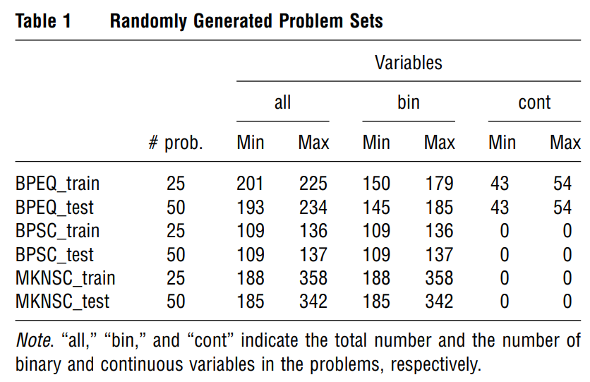
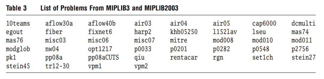
two types of problem sets, namely randomly generated problem setsandstandard benchmark problemsfrom the MIPLIB.The random problem sets are used for both training (steps 1 and 2) and assessing (step 3) the heuristics. MIPLIB problems are only used for assessment (step 3).
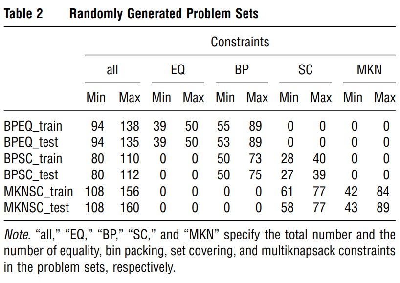
The possible constraints are chosen among set covering (SC), multiknapsack (MKN), bin packing (BP), and equality (EQ) constraints. We generated problems that contain constraints of type BP-EQ, BP-SC, and MKN-SC.
As some of those problems are going to be used to generate the training data set, we randomly split each family into a train and a test set. In the end, we have six data sets: BPEQ_train, BPEQ_test, BPSC_train, BPSC_test, MKNSC_train, and MKNSC_test.
The chosen parameters of ExtraTrees are , and .
4.3 Results
We compare our approach to five other branching strategies, namely random branching (random), most-infeasible branching (MIB), nonchimerical branching (NCB) (Fischetti and Monaci 2012), full strong branching (FSB), and reliability branching (RB) (Achterberg et al. 2005).
In these tables (Tables 4, 5, and 7), Cl. Gap refers to the closed gap and S/T indicates the number of problems solved within the provided nodes or time limit versus the total number of problems. Nodes and Time, respectively, represent the number of explored nodes and the time spent (in seconds) before the optimization either finds the optimal solution or stops earlier because of one stopping criterion.
The normal learned branching strategy (i.e., (, all)) is learned based on a data set containing samples from the three types of training problems (i.e., BPSC, BPEQ, and MKNSC).

Those results show that our approach succeeds in efficiently imitating FSB. Indeed, the experiments performed with a limit on the number of nodes show that the closed gap is only 9% smaller, while the time spent is reduced by 85% compared to FSB. The experiments with a time limit show that the reduced time required to take a decision allows the learned strategy to explore more nodes and to thus further close the gap than FSB. While these results are encouraging, they are still slightly worse than the results obtained with RB, which is both closer to FSB and faster than our approach
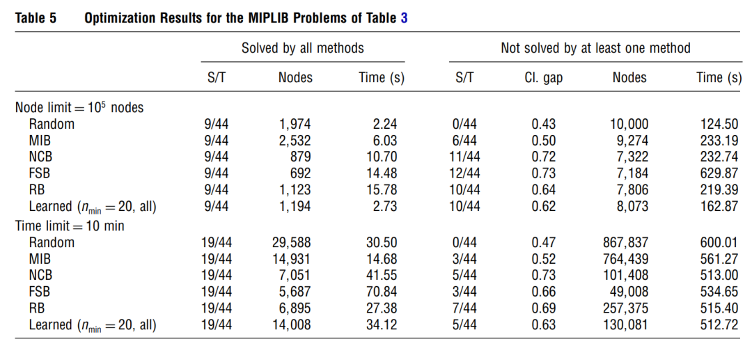
we separated the problems that were solved by all methods from the problems that were not solved by at least one of the compared methods. the results obtained with the learned branching strategy are still a little below the results obtained with reliability branching. The results presented here are averaged over all considered problems.
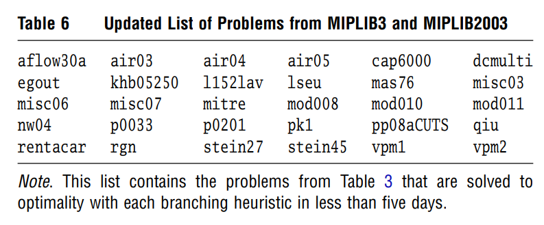
Finally, Tables 6 and 7 report the results form our last set of experiments.
Additionally, in another experiment, we let CPLEX use cuts and heuristics (with default CPLEX parameters) in the course of the optimization to observe their impact on the efficiency of each branching strategy.

Overall, our method compares favorably to its competitors when cuts and heuristics are used by CPLEX. Indeed, in that case, our learned branching strategy is the fastest (almost three times faster than the second fastest method (i.e., MIB)) to solve all 30 considered problems.
Note that the apparent bad results of RB are due to three problems that are especially hard for that branching heuristic (air04, air05, and mod011).
Things appear to be different when cuts and heuristics are not used. Indeed, based on the results of Table 7, our method seems to be very slow, but the large number of nodes and the large amount of time is actually due to a small number of problems for which the method does not work well.
A possible explanation for why our method does not perform well on those problems can be that these problems, because too large, are not well represented in the data set that we use to learn the branching strategy.
Reference
[1] Alejandro Marcos Alvarez, Quentin Louveaux, Louis Wehenkel (2017) A Machine Learning-Based Approximation of Strong Branching. INFORMS Journal on Computing 29(1):185-195. http://dx.doi.org/10.1287/ijoc.2016.0723
推薦閱讀:
干貨 | 想學(xué)習(xí)優(yōu)化算法,不知從何學(xué)起?
干貨 | 運(yùn)籌學(xué)從何學(xué)起?如何快速入門運(yùn)籌學(xué)算法?
干貨 | 學(xué)習(xí)算法,你需要掌握這些編程基礎(chǔ)(包含JAVA和C++)
干貨 | 算法學(xué)習(xí)必備訣竅:算法可視化解密
