
Learning to Solve Security-Constrained Unit Commitment Problems
論文閱讀筆記,個人理解,如有錯誤請指正,感激不盡!該文分類到Machine learning alongside optimization algorithms。
01 Security-constrained unit commitment (SCUC)基于安全約束的機組組合優(yōu)化 (Security-constrained unit commitment, SCUC) 是能源系統(tǒng)和電力市場中一個基礎的問題。機組組合在數(shù)學上是一個包含0-1整型變量和連續(xù)變量的高維,離散,非線性混合整數(shù)優(yōu)化問題。
簡單點說呢,就是需要對發(fā)電機組進行決策,決定哪些發(fā)電機開哪些關,以及開的發(fā)電機生產(chǎn)多少電力,從而滿足市場的需求。目標是使得發(fā)電總成本最小化(當然也有很多其他目標,比如考慮環(huán)境影響)。約束主要是要確保安全約束,即每一條傳輸電的線路,傳輸?shù)碾娏坎荒艹^其負荷。當然小編這方面可能不是很專業(yè),詳細描述請看文獻或者咨詢電氣專業(yè)的比較合適。
考慮一個能源系統(tǒng),定義如下的參數(shù)集合:
- 為公交車集合(消耗電的)
- 為發(fā)電機集合
- 為線路的集合
- 為一個時長周期
對于每一個發(fā)電機和每一個小時,定義如下的決策變量:
- 為一個0-1變量,表示發(fā)電機在時間是否開啟
- 為連續(xù)的變量,表示發(fā)電機在時間所產(chǎn)生的電量
構(gòu)建SCUC的模型如下(完整模型請參考文獻Appendix):
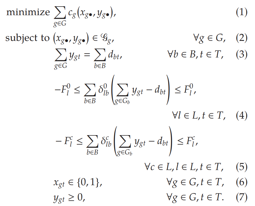
In the objective function, is a piecewise-linear function that includes the startup, shutdown, and production costs for generator . The notation is a shorthand for the vector , where .
Constraint (2)enforces a number of constraints that are local for each generator, including production limits, minimum-up and minimum-down running times, and ramping rates, among others.Constraint (3)enforces that the total amount of power produced equals the sum of the demands at each bus.Constraint (4)enforces the deliverability of power under normal system conditions. The set denotes the set of generators attached to bus . where are real numbers known as injection shift factors (ISFs). Let be its flow limit (in megawatt-hours) under normal conditions and be its flow limit when there is an outage online .Constraints (5)enforce the deliverability of power under the scenario that line has had an outage. The bounds and the ISFs may be different under each outage scenario.
上面的模型中,一個比較顯著的特點是,Constraint (4)和Constraints (5) (Transmission Constraints) 對模型的求解有著非常關鍵的影響。這兩個約束的數(shù)量是傳輸路線數(shù)的平方,而大型的能源一般擁有超過10000條的傳輸線路,這樣一來,兩個約束的總數(shù)量就可能超過一億了。
To make matters worse, these constraints are typically very dense, which makes adding them all to the formulation impractical for large-scale instances not only because of degraded MIP performance but also because of memory requirements.
Fortunately, it has been observed that enforcing only a very small subset of these constraints is already sufficient to guarantee that all the remaining constraints are automatically satisfied.
02 Setting and Learning Strategies上面已經(jīng)介紹了SCUC的模型以及模型的一些特點。目前求解SCUC的方法還是MIP (Mixed-Integer Programming) 為主,但是由于前面提到的難點,MIP在大規(guī)模問題上的表現(xiàn)一般。基于此,作者在文章中結(jié)合machine learning (ML) 提出了一種新的優(yōu)化框架,該框架主要包含了三個ML的模型:
- The first model is designed to predict, based on statistical data, which constraints are necessary in the formulation and which constraints can be safely omitted.
- The second model constructs, based on a large number of previously obtained optimal solutions, a (partial) solution that is likely to work well as a warm start.
- The third model identifies,with very high confidence, a smaller-dimensional affine subspace where the optimal solution is likely to lie, leading to the elimination of a large number of decision variables and significantly reducing the complexity of the problem.
在開始之前,先介紹一些設置的參數(shù)。Assume that every instance of SCUC is completely described by a vector of real-valued parameters . These parameters include only the data that are unknown to the market operators the day before the market-clearing process takes places. For example, they may include the peak system demand and the production costs for each generator. In this work, we assume that network topology and the total number of generators are known ahead of time, so there is no need to encode them via parameters. We may therefore assume that , where is fixed. We are given a set of training instances that are similar to the instance we expect to solve during actual market clearing.
2.1 Learning Violated Transmission Constraints
如同前面提到的,求解SCUC的MIP時,較大的挑戰(zhàn)就是如何處理數(shù)量巨大的Transmission Constraints,即模型中的Constraint (4)和Constraints (5)。因此第一個ML model要做的就是預測哪些Transmission Constraints需要在初始時就添加到SCUC的relaxation中而哪些又可以直接忽略(即這些約束不會被違背)。
在此之前,作者先使用了Xavier et al. (2019)其實就是他自己。。。提出的一個有效求解SCUC的iterative contingency screening algorithm:
The method works by initially solving a relaxed version of SCUC where no transmission or N ? 1 security constraints are enforced. At each iteration, all violated constraints are identified, but only a small and carefully selected subset is added to the relaxation. The method stops when no further violations are detected, in which case the original problem is solved.
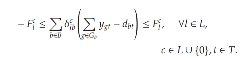
基于此,作者修改了上面的方法,加入了一個ML predictor。令為傳輸線的集合,模型中關于Transmission Constraints如下:
假設定制的MIP solver接受來自ML predictor的指示:
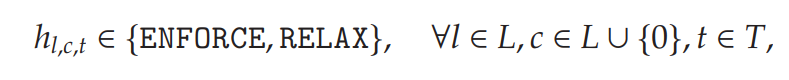
indicating whether the thermal limits of transmission line , under contingency scenario (normal?conditions對應約束(4),而outage?online對應約束(5) ), at time t, are likely to be binding in the optimal solution. Given these hints, the solver proceeds as described in Algorithm 1.
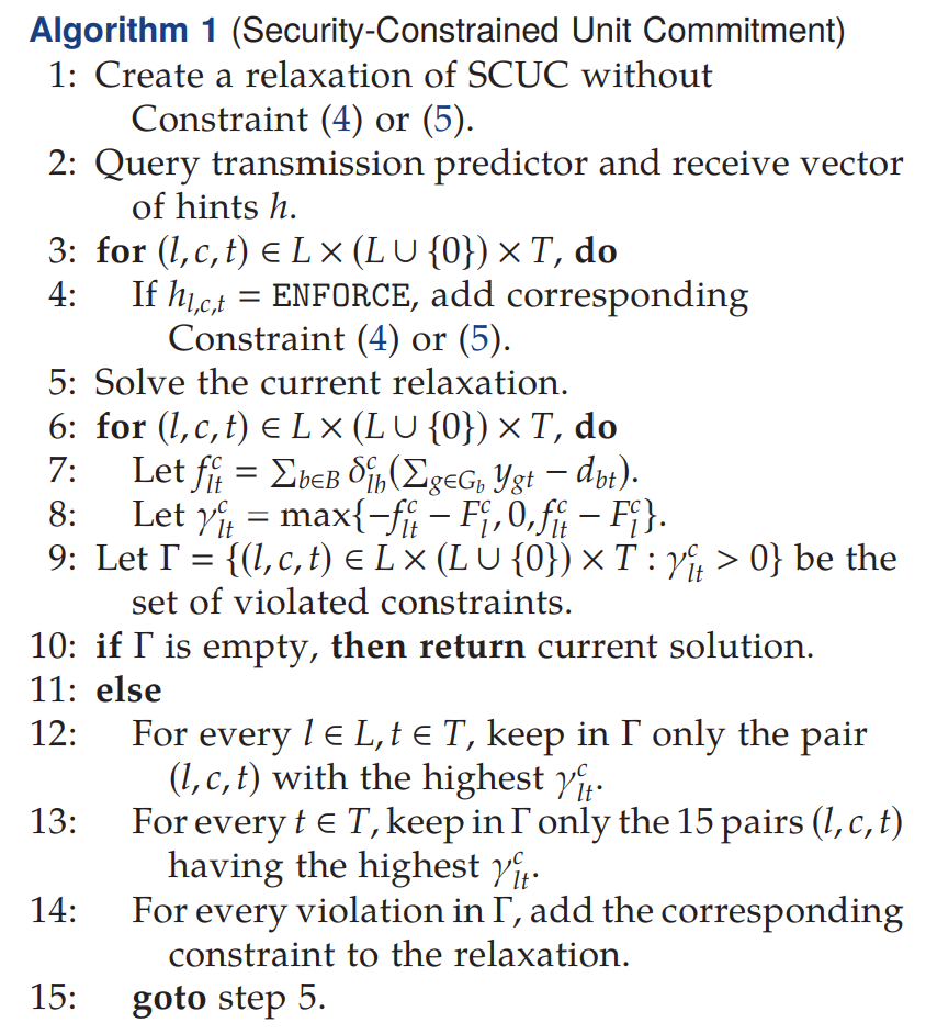
In the first iteration, only the transmission constraints specified by the hints are enforced. For the remaining iterations, the solver follows exactly the same strategy as the baseline method and keeps adding small subsets of violated constraints until no further violations are found.
If the predictor is successful and correctly predicts a superset of the binding transmission constraints, then only one iteration is necessary for the algorithm to converge.
If the predictor fails to identify some necessary constraints, the algorithm may require additional iterations but still returns the correct solution.
For this prediction task, we propose a simple learning strategy based on kNN. Let be the training parameters. During training, the instances are solved using Algorithm 1, where the initial hints are set to RELAX for all constraints. During the solution of each training instance , we record the set of constraints that was added to the relaxation by Algorithm 1. During the test, given a vector of parameters , the predictor finds a list of k vectors that are the closest to and sets = ENFORCE if appears in at least p% of the sets , where p is a hyperparameter.
本文設置,因為少添加一個正確的Transmission Constraints所來帶的損失要比多添加一堆不正確的Transmission Constraints要低得多(少添加后面加回去就行了,而多添加了,每次都slow down模型的求解速度)。
2.2 Learning Warm Starts
求解SCUC的另一個挑戰(zhàn)就是如何獲得高質(zhì)量的可行初始解,作者吸收了很多文獻中的方法的精髓。Our aim is to produce, based on a large number of previous optimal solution, a (partial) solution that works well as a warm start.
Let be the training parameters, and let be their optimal solutions. In principle, the entire list of solutions could be provided as warm starts to the solver.
We propose instead the use of kNN to construct a single (partial and possibly infeasible) solution, which should be repaired by the solver. The idea is to set the values only for the variables that we can predict with high confidence and to let the MIP solver determine the values for all the remaining variables. To maximize the likelihood of our warm starts being useful, we focus on predicting values for the binary variables ; all continuous variables are determined by the solver.
Given a test parameter , first we find the k solutions corresponding to the k nearest training instances .
Then, for each variable , we verify the average of the values . If , where is a hyperparameter, then the predictor sets to 1 in the warm start solution. If , then the value is set to 0. In any other case, the value is left undefined.
2.3 Learning Affine Subspaces
在實際的操作中,工人憑借著以往的經(jīng)驗,知道很多特征。比如,他們知道每天有多少電量必然會被消耗的,人工操作的時候,這些是非常顯而易見的。但是,一旦建模成MIP,利用solver來求解的時候,這些就完全丟掉了。
Given the fixed characteristics of a particular power system and a realistic parameter distribution, new constraints probably could be safely added to the MIP formulation of SCUC to restrict its solution space without affecting its set of optimal solutions. In this subsection, we develop a ML model for finding such constraints automatically, based on statistical data.
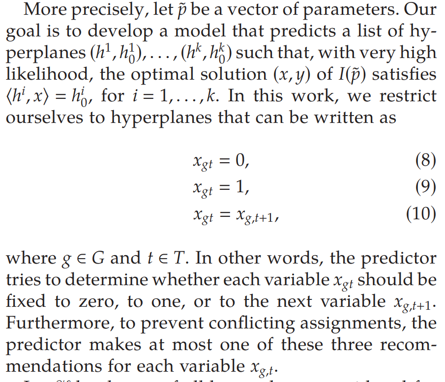
文中沒有給出的具體含義,小編猜想應該是對應的是中的gt,即哪些變量;而對應的是的取值,即上面的式子(8)、(9)、(10)。這個模型的主要功能是通過添加上面的約束,進一步限制解的空間,從而加快算法的速度。但是得保證,砍掉的那部分不會出現(xiàn)在最優(yōu)解中。更詳細的描述請看論文。
03 Computational Experiments測試算例以下網(wǎng)址可以獲得:
https://zenodo.org/record/3648686
3.1 Evaluation of Transmission Predictor
zerocorresponds to the case where no ML is used.tr:nearest, we add to the initial relaxation all constraints that were necessary during the solution of the most similar training variation.tr:all, we add all constraints that were ever necessary during training.tr:knn:kcorrespond to the method outlined in Section 3.1, where is the hyperparameter describing the number of neighbors.tr:perfshows the performance of the theoretically perfect predictor, which can predict the exact set of constraints found by the iterative method, with perfect accuracy, under zero running time.
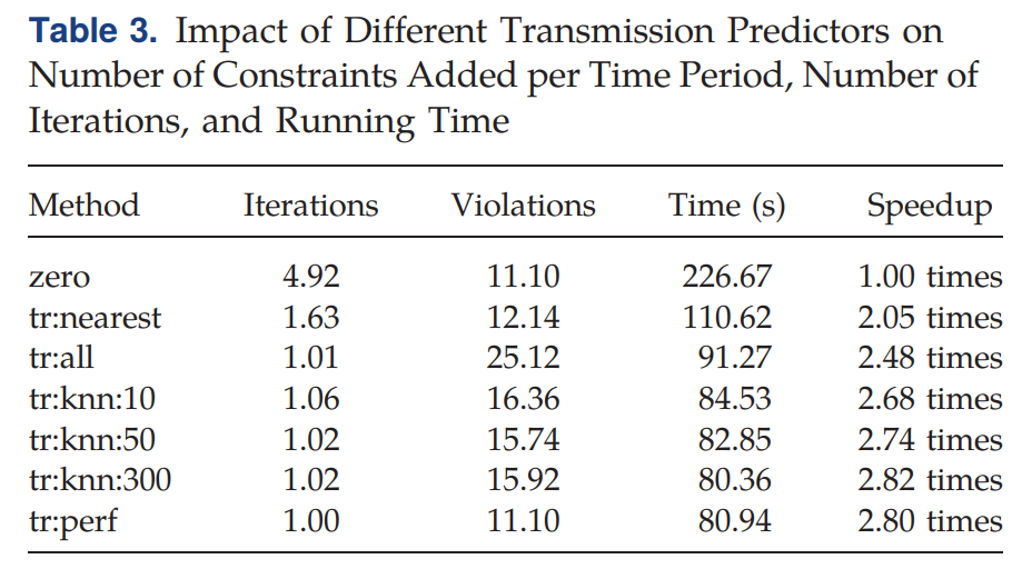
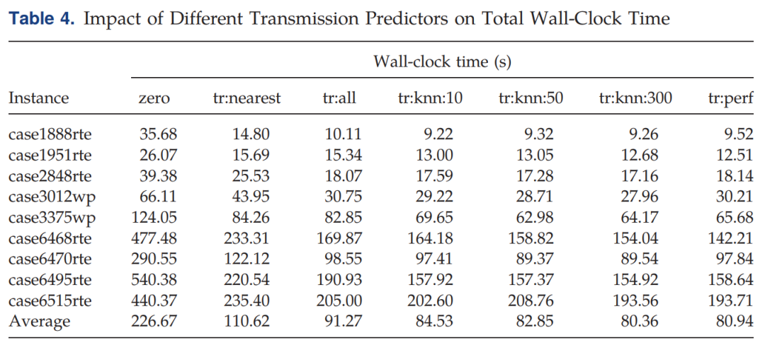
以zero為基準,使用了ML的基本速度都快了2-3倍不等。
3.2 Evaluation of the Warm-Start Predictor
Strategy tr:knn:300, as introduced in Section 4.3, is included as a baseline and only predicts transmission constraints and not warm starts. All other strategies presented in this section are built on top of tr:knn:300; that is, prediction of transmission constraints is performed first, using tr:knn:300, and then prediction of warm starts is performed.
In strategies ws:collect:n, we provide to the solver warm starts, containing the optimal solutions of the nearest training variations.
Strategies ws:knn:k : p, for and , correspond to the strategy described in Section 3.2.
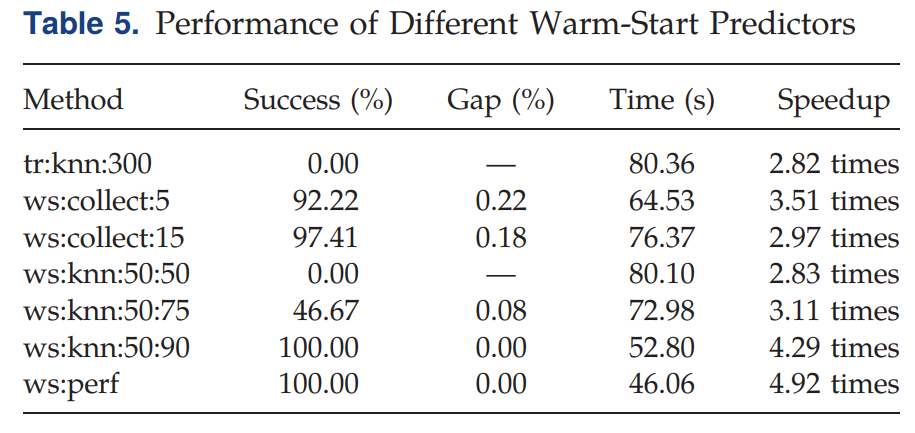
在Table 5中:
- Success(%): 表示W(wǎng)arm-Start Predictor給出一個可行解的成功率
- Gap (%): 表示W(wǎng)arm-Start Predictor給出的解和最優(yōu)解的差距,越低越好,為0表示W(wǎng)arm-Start Predictor初始時給出了最優(yōu)解。
- Time (s): 求解時間
Table 6中的tr:knn:50寫錯了,應該是tr:knn:300。。。
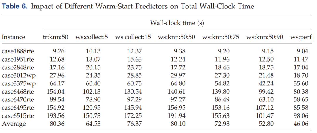
可以看到,結(jié)合第一個model,加了Warm-Start Predictor以后,速度有顯著提升,相對于tr:knn:300.
3.3 Evaluation of the Affine Subspace Predictor
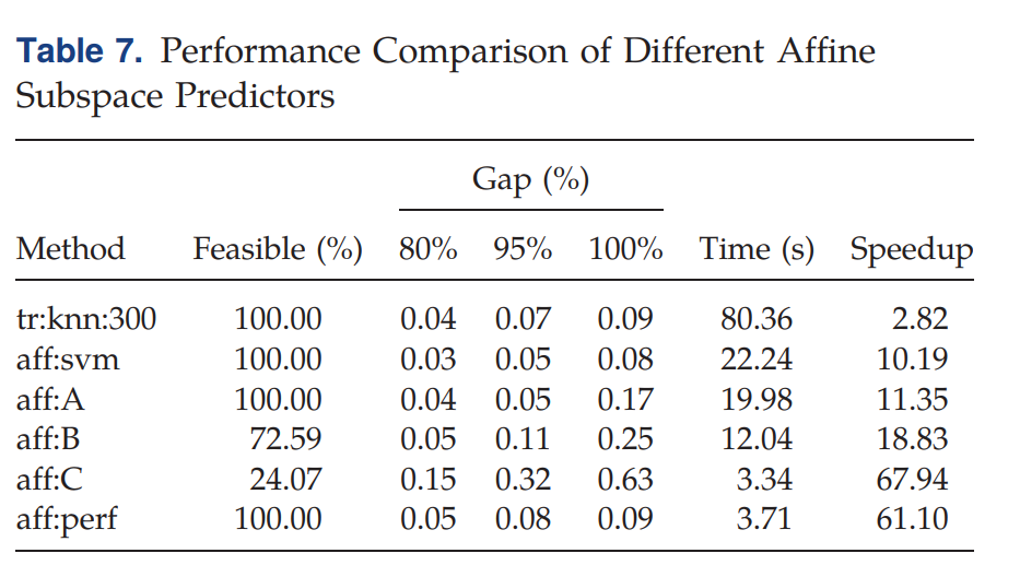
同樣, Method tr:knn:300 is the kNN predictor for transmission constraints. This predictor does not add any hyperplanes to the relaxation and is used only as a baseline. All the following predictors were built on top of tr:knn:300.
幾個aff:的Predictor不同主要在于內(nèi)部設置的一些參數(shù)不同,詳細看論文好了。在Table 7中:
- Feasible (%): 表示加了該hyperplanes以后(即縮小了解空間),所生成的解可行的百分比
- Gap (%): 以95%下的0.07為例,表示有95%的問題變體(加入hyperplanes以后)得出來的gap與最優(yōu)解相差0.07
Four different strategies are presented: no ML (0), transmission prediction (tr:knn:300), transmission plus warm-start prediction (ws:knn:50:90), and transmission plus affine subspace prediction (aff:svm).
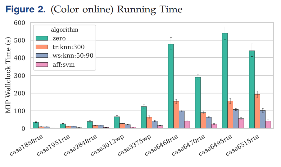
可以看到aff:svm的時間是最短的。Overall, using different ML strategies, we were able to obtain a 4.3 times speedup while maintaining optimality guarantees (ws:knn:50:90) and a 10.2 times speedup without guarantees but with no observed reduction in solution quality (aff:svm).
[1] álinson S. Xavier, Feng Qiu, Shabbir Ahmed (2020) Learning to Solve Large-Scale Security-Constrained Unit Commitment Problems. INFORMS Journal on Computing
推薦閱讀:
干貨 | 學習算法,你需要掌握這些編程基礎(包含JAVA和C++)
記得點個在看支持下哦~
