
【小白學(xué)習(xí)Keras教程】四、Keras基于數(shù)字?jǐn)?shù)據(jù)集建立基礎(chǔ)的CNN模型
「@Author:Runsen」
加載數(shù)據(jù)集
1.創(chuàng)建模型
2.卷積層
3. 激活層
4. 池化層
5. Dense(全連接層)
6. Model compile & train
基本卷積神經(jīng)網(wǎng)絡(luò)(CNN)
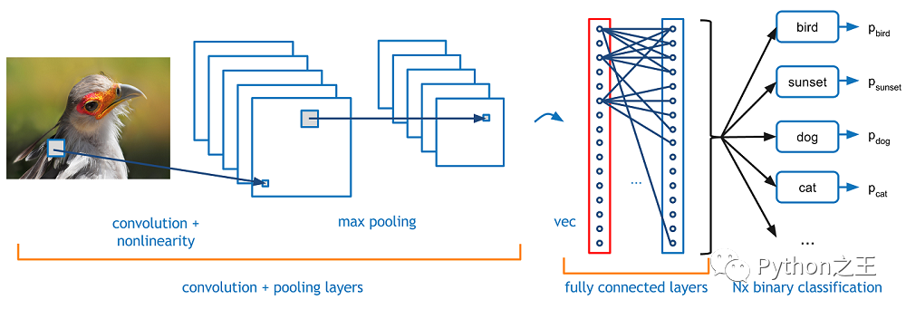
-CNN的基本結(jié)構(gòu):CNN與MLP相似,因?yàn)樗鼈冎幌蚯皞魉托盘?hào)(前饋網(wǎng)絡(luò)),但有CNN特有的不同類型的層
「Convolutional layer」:在一個(gè)小的感受野(即濾波器)中處理數(shù)據(jù) 「Pooling layer」:沿2維向下采樣(通常為寬度和高度) 「Dense (fully connected) layer」:類似于MLP的隱藏層
import numpy as np
import matplotlib.pyplot as plt

from sklearn import datasets
from sklearn.model_selection import train_test_split
from keras.utils.np_utils import to_categorical
加載數(shù)據(jù)集
sklearn中的數(shù)字?jǐn)?shù)據(jù)集 文檔:http://scikit-learn.org/stable/auto_examples/datasets/plot_digits_last_image.html
data = datasets.load_digits()
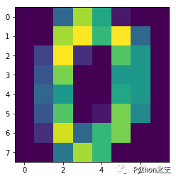
plt.imshow(data.images[0]) # show first number in the dataset
plt.show()
print('label: ', data.target[0]) # label = '0'
X_data = data.images
y_data = data.target
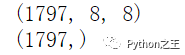
# shape of data
print(X_data.shape) # (8 X 8) format
print(y_data.shape)
# reshape X_data into 3-D format
X_data = X_data.reshape((X_data.shape[0], X_data.shape[1], X_data.shape[2], 1))
# one-hot encoding of y_data
y_data = to_categorical(y_data)
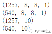
將數(shù)據(jù)劃分為列車(chē)/測(cè)試集
X_train, X_test, y_train, y_test = train_test_split(X_data, y_data, test_size = 0.3, random_state = 777)
print(X_train.shape)
print(X_test.shape)
print(y_train.shape)
print(y_test.shape)
from keras.models import Sequential
from keras import optimizers
from keras.layers import Dense, Activation, Flatten, Conv2D, MaxPooling2D
1.創(chuàng)建模型
創(chuàng)建模型與MLP(順序)相同
model = Sequential()
2.卷積層
通常,二維卷積層用于圖像處理 濾波器的大小(由“kernel\u Size”參數(shù)指定)定義感受野的寬度和高度** 過(guò)濾器數(shù)量(由“過(guò)濾器”參數(shù)指定)等于下一層的「深度」 步幅(由“步幅”參數(shù)指定)是「過(guò)濾器每次移動(dòng)改變位置」的距離 圖像可以「零填充」以防止變得太小(由“padding”參數(shù)指定) Doc: https://keras.io/layers/convolutional/
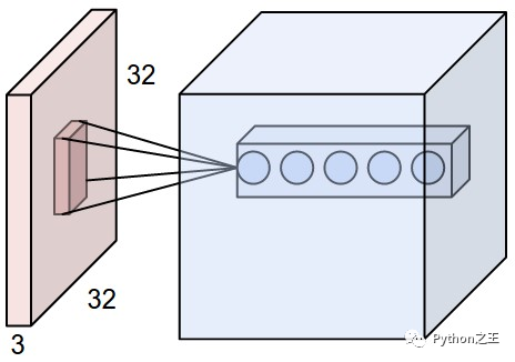
# convolution layer
model.add(Conv2D(input_shape = (X_data.shape[1], X_data.shape[2], X_data.shape[3]), filters = 10, kernel_size = (3,3), strides = (1,1), padding = 'valid'))
3. 激活層
與 MLP 中的激活層相同 一般情況下,也使用relu Doc: http://cs231n.github.io/assets/cnn/depthcol.jpeg
model.add(Activation('relu'))
4. 池化層
一般使用最大池化方法 減少參數(shù)數(shù)量 文檔:https://keras.io/layers/pooling/
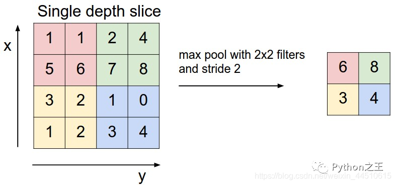
model.add(MaxPooling2D(pool_size = (2,2)))
5. Dense(全連接層)
卷積和池化層可以連接到密集層 文檔:https://keras.io/layers/core/
# prior layer should be flattend to be connected to dense layers
model.add(Flatten())
# dense layer with 50 neurons
model.add(Dense(50, activation = 'relu'))
# final layer with 10 neurons to classify the instances
model.add(Dense(10, activation = 'softmax'))
6. Model compile & train
adam = optimizers.Adam(lr = 0.001)
model.compile(loss = 'categorical_crossentropy', optimizer = adam, metrics = ['accuracy'])
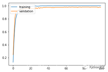
history = model.fit(X_train, y_train, batch_size = 50, validation_split = 0.2, epochs = 100, verbose = 0)
plt.plot(history.history['acc'])
plt.plot(history.history['val_acc'])
plt.legend(['training', 'validation'], loc = 'upper left')
plt.show()
results = model.evaluate(X_test, y_test)
print('Test accuracy: ', results[1])

公眾號(hào)后臺(tái)回復(fù)《資料》可以獲得對(duì)應(yīng)的大量Python筆記和手冊(cè)
評(píng)論
圖片
表情