論文閱讀筆記，個(gè)人理解，如有錯(cuò)誤請(qǐng)指正，感激不盡！僅是對(duì)文章進(jìn)行梳理，細(xì)節(jié)請(qǐng)閱讀參考文獻(xiàn)。該文分類到Machine learning alongside optimization algorithms。

01 Column Generation

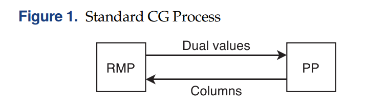
列生成 (Column Generation) 算法在組合優(yōu)化領(lǐng)域有著非常廣泛的應(yīng)用，是一種求解大規(guī)模問(wèn)題 (large-scale optimization problems) 的有效算法。在列生成算法中，將大規(guī)模線性規(guī)劃問(wèn)題分解為主問(wèn)題 (Master Problem, MP) 和定價(jià)子問(wèn)題 (Pricing Problem, PP)。算法首先將一個(gè)MP給restricted到只帶少量的columns，得到RMP。求解RMP，得到dual solution，并將其傳遞給PP，隨后求解PP得到相應(yīng)的column將其加到RMP中。RMP和PP不斷迭代求解直到再也找不到檢驗(yàn)數(shù)為負(fù)的column，那么得到的RMP的最優(yōu)解也是MP的最優(yōu)解。如下圖所示：

關(guān)于列生成的具體原理，之前已經(jīng)寫過(guò)很多詳細(xì)的文章了。還不熟悉的小伙伴可以看看以下：

干貨 | 10分鐘帶你徹底了解Column Generation（列生成）算法的原理附j(luò)ava代碼

干貨 | 10分鐘教你使用Column Generation求解VRPTW的線性松弛模型

干貨 | 求解VRPTW松弛模型的Column Generation算法的JAVA代碼分享

02 Column Selection

在列生成迭代的過(guò)程中，有很多技巧可以用來(lái)加快算法收斂的速度。其中一個(gè)就是在每次迭代的時(shí)候，加入多條檢驗(yàn)數(shù)為負(fù)的column，這樣可以減少迭代的次數(shù)，從而加快算法整體的運(yùn)行時(shí)間。特別是求解一次子問(wèn)題得到多條column和得到一條column相差的時(shí)間不大的情況下（例如，最短路中的labeling算法）。

而每次迭代中選擇哪些column加入？是一個(gè)值得研究的地方。因?yàn)榧尤氲腸olumns不同，最終收斂的速度也大不一樣。一方面，我們希望加入column以后，目標(biāo)函數(shù)能盡可能降低（最小化問(wèn)題）；另一方面，我們希望加入的column數(shù)目越少越好，太多的列會(huì)導(dǎo)致RMP求解難度上升。因此，在每次的迭代中，我們構(gòu)建一個(gè)模型，用來(lái)選擇一些比較promising的column加入到RMP中：

Let be the CG iteration number
the set of columns present in the RMP at the start of iteration
the generated columns at this iteration
For each column , we define a decision variable that takes value one if column is selected and zero otherwise

為了最小化所選擇的column，每選擇一條column的時(shí)候，都會(huì)發(fā)生一個(gè)足夠小的懲罰。最終，構(gòu)建column selection的模型 (MILP) 如下：

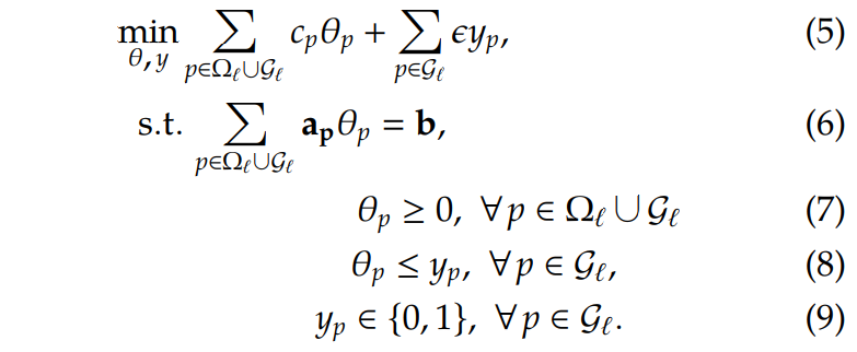
大家發(fā)現(xiàn)沒(méi)有，如果沒(méi)有和約束(8)和(9)，那么上面這個(gè)模型就直接變成了下一次迭代的RMP了。

假設(shè)足夠小，這些約束目的是使得被選中添加到RMP中的column數(shù)量最小化，也就是這些的columns。那么在迭代中要添加到RMP的的column為：

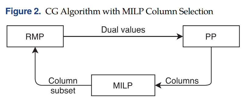
總體的流程如下圖所示：

03 Graph Neural Networks

在每次迭代中，通過(guò)求解MILP，可以知道加入哪些column有助于算法速度的提高，但是求解MILP也需要一定的時(shí)間，最終不一定能達(dá)到加速的目的。因此通過(guò)機(jī)器學(xué)習(xí)的方法，學(xué)習(xí)一個(gè)MILP的模型，每次給出選中的column，將是一種比較可行的方法。

在此之前，先介紹一下Graph Neural Networks。圖神經(jīng)網(wǎng)絡(luò)（GNNs）是通過(guò)圖節(jié)點(diǎn)之間的信息傳遞來(lái)獲取圖的依賴性的連接模型。與標(biāo)準(zhǔn)神經(jīng)網(wǎng)絡(luò)不同，圖神經(jīng)網(wǎng)絡(luò)可以以任意深度表示來(lái)自其鄰域的信息。

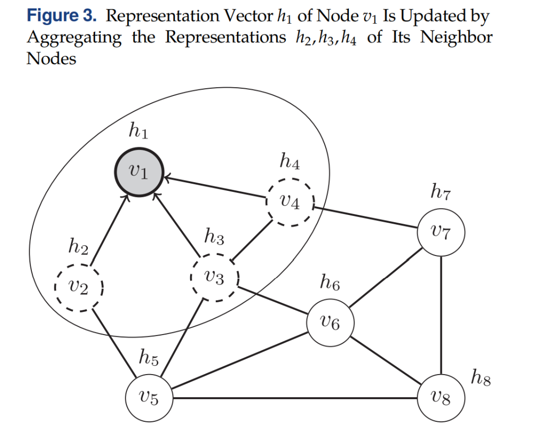
給定一個(gè)網(wǎng)絡(luò)，其中是頂點(diǎn)集而是邊集。每一個(gè)節(jié)點(diǎn)有著特征向量。目的是迭代地aggregate（聚合）相鄰節(jié)點(diǎn)的信息以更新節(jié)點(diǎn)的狀態(tài)，令：

be the representation vector of node （注意和區(qū)分開(kāi)）at iteration
Let be the set of neighbor (adjacent) nodes of

如下圖所示，節(jié)點(diǎn)從相鄰節(jié)點(diǎn) aggregate信息來(lái)更新自己：

在迭代中，一個(gè)aggregated function，記為，在每個(gè)節(jié)點(diǎn)上首先用于計(jì)算一個(gè)aggregated information vector :

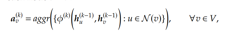
其中在初始時(shí)有，是一個(gè)學(xué)習(xí)函數(shù)。應(yīng)該和節(jié)點(diǎn)順序無(wú)關(guān)，例如sum, mean, and min/max functions。

接著，使用另一個(gè)函數(shù)，記為，將aggregated information與節(jié)點(diǎn)當(dāng)前的狀態(tài)進(jìn)行結(jié)合，更新后的節(jié)點(diǎn)representation vectors:

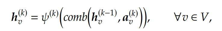
其中是另一個(gè)學(xué)習(xí)函數(shù)。在不斷的迭代中，每一個(gè)節(jié)點(diǎn)都收集來(lái)自更遠(yuǎn)鄰居節(jié)點(diǎn)的信息，在最后的迭代中，節(jié)點(diǎn)的 representation 就可以用來(lái)預(yù)測(cè)其標(biāo)簽值了，使用最后的轉(zhuǎn)換函數(shù)（記為），最終：

04 A Bipartite Graph for Column Selection

利用上面的GNN來(lái)做Column Selection，比較明顯的做法是一個(gè)節(jié)點(diǎn)表示一個(gè)column，然后將兩個(gè)column通過(guò)一條邊連接如果他們都與某個(gè)約束相關(guān)聯(lián)的話。但是這樣會(huì)導(dǎo)致大量的邊，并且對(duì)偶值的信息也很難在模型中進(jìn)行表示。

因此作者使用了bipartite graph with two node types：column nodes and constraint nodes . An edge exists between a node and a node if column contributes to constraint . 這樣做的好處是可以在節(jié)點(diǎn)上附加特征向量，例如對(duì)偶解的信息，如下圖(a)所示：

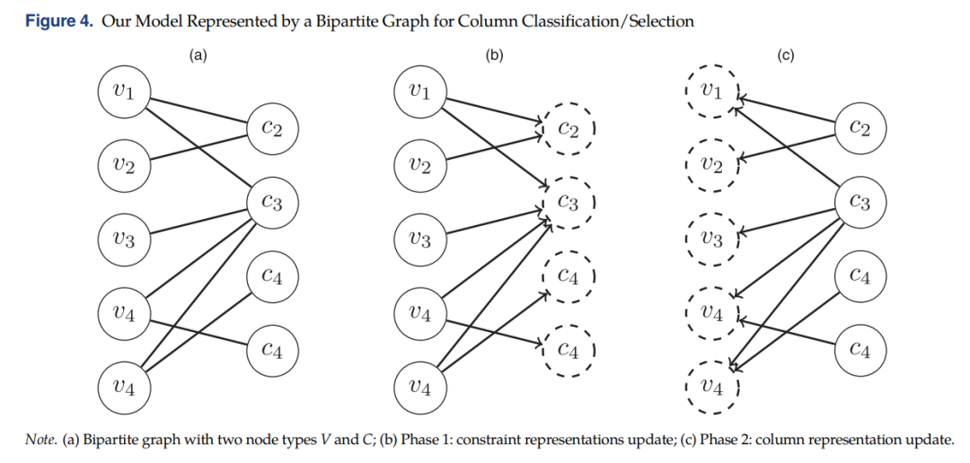
因?yàn)橛袃煞N類型的節(jié)點(diǎn)，每一次迭代時(shí)均有兩階段：階段1更新Constraint節(jié)點(diǎn)(上圖(b))，階段2更新Column節(jié)點(diǎn)(上圖(c))。最終，column節(jié)點(diǎn)的 representations 被用來(lái)預(yù)測(cè)節(jié)點(diǎn)的labels 。算法的流程如下：

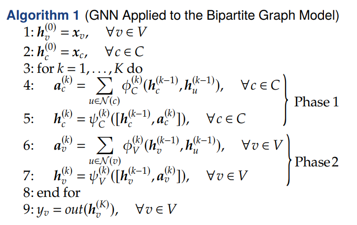
As described in the previous section, we start by initializing the representation vectors of both the column and constraint nodes by the feature vectors and , respectively (steps 1 and 2). For each iteration , we perform the two phases: updating the constraint representations (steps 4 and 5), then the column ones (steps 6 and 7). The sum function is used for the aggr function and the vector concatenation for the comb function.

The functions , and are two-layer feed forward neural networks with rectified linear unit (ReLU) activation functions and out is a three-layer feed forward neural network with a sigmoid function for producing the final probabilities (step 9).

A weighted binary cross entropy loss is used to evaluate the performance of the model, where the weights are used to deal with the imbalance between the two classes. Indeed, about 90% of the columns belong to the unselected class, that is, their label .

05 數(shù)據(jù)采集

數(shù)據(jù)通過(guò)使用前面提到的MILP求解多個(gè)算例來(lái)采集column的labels。每次的列生成迭代都將構(gòu)建一個(gè)Bipartite Graph并且存儲(chǔ)以下的信息：

The sets of column and constraint nodes;
A sparse matrix storing the edges;
A column feature matrix , where is the number of columns and d the number of column features;
A constraint feature matrix , where is the number of constraints and the number of constraint features;
The label vector y of the newly generated columns in .

06 Case Study I: Vehicle and Crew Scheduling Problem

關(guān)于這個(gè)問(wèn)題的定義就不寫了，大家可以自行去了解一下。

6.1 MILP Performance

通過(guò)刻畫在列生成中使用MILP和不使用MILP(所有生成的檢驗(yàn)數(shù)為負(fù)的column都丟進(jìn)下一次的RMP里)的收斂圖如下：

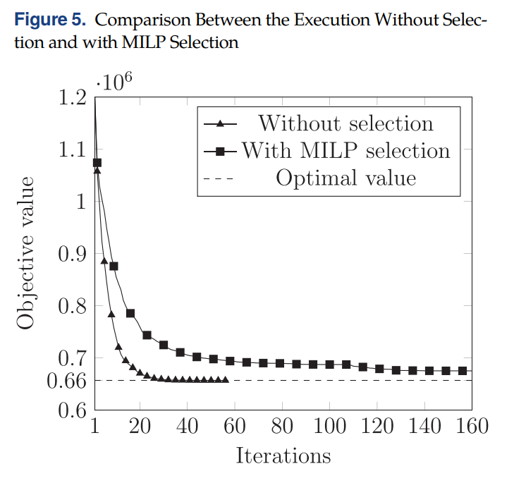
使用了MILP收斂速度反而有所下降，This is mainly due to the rejected columns that remain with a negative reduced cost after the RMP reoptimization and keep on being generated in subsequent iterations, even though they do not improve the objective value (degeneracy).

為了解決這個(gè)問(wèn)題，一個(gè)可行的方法是運(yùn)行MILP以后，額外再添加一些column。不過(guò)是先將MILP選出來(lái)的column加進(jìn)RMP，進(jìn)行求解，得到duals以后，再去未被選中的column中判斷，哪些column在新的duals下檢驗(yàn)數(shù)依然為負(fù)，然后進(jìn)行添加。當(dāng)然，未選中的column過(guò)多的話，不一定把所有的都加進(jìn)去，按照檢驗(yàn)數(shù)排序，加一部分就好（該文是50%）。如下圖所示：

加入了額外的column以后，在進(jìn)行preliminary的測(cè)試，結(jié)果如下(the computational time of the algorithm with column selection does not include the time spent solving the MILP at every iteration，因?yàn)樽髡咧幌肓私鈙election對(duì)column generation的影響，反正MILP最后要被更快的GNN模型替代的。)：

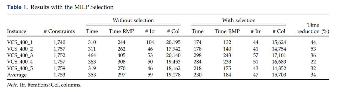
可以看到，MILP能節(jié)省更多的計(jì)算時(shí)間，減少約34%的總體時(shí)間。

6.2 Comparison

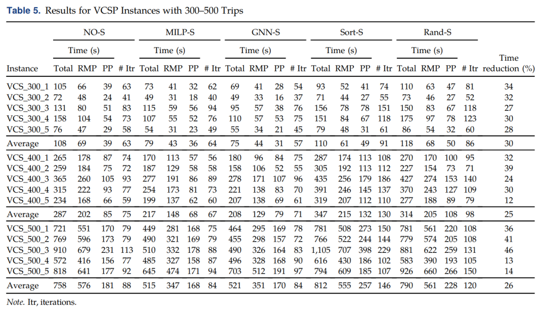
隨后，對(duì)以下的策略進(jìn)行對(duì)比：

No selection (NO-S): This is the standard CG algorithm with no selection involved, with the use of the acceleration strategies described in Section 2.
MILP selection (MILP-S): The MILP is used to select the columns at each iteration, with 50% additional columns to avoid convergence issues. Because the MILP is considered to be the expert we want to learn from and we are looking to replace it with a fast approximation, the total computational time does not include the time spent solving the MILP.
GNN selection (GNN-S): The learned model is used to select the columns. At every CG iteration, the column features are extracted, the predictions are obtained, and the selected columns are added to the RMP.
Sorting selection (Sort-S): The generated columns are sorted by reduced cost in ascending order, and a subset of the columns with the lowest reduced cost are selected. The number of columns selected is on average the same as with the GNN selection.
Random selection (Rand-S): A subset of the columns is selected randomly. The number of columns selected is on average the same as with the GNN selection

對(duì)比的結(jié)果如下，其中The time reduction column compares the GNN-S to the NO-S algorithm.相比平均減少26%的時(shí)間。

07 Case Study II: Vehicle Routing Problem with Time Windows

這是大家的老熟客了，就不過(guò)多介紹了。直接看對(duì)比的結(jié)果：

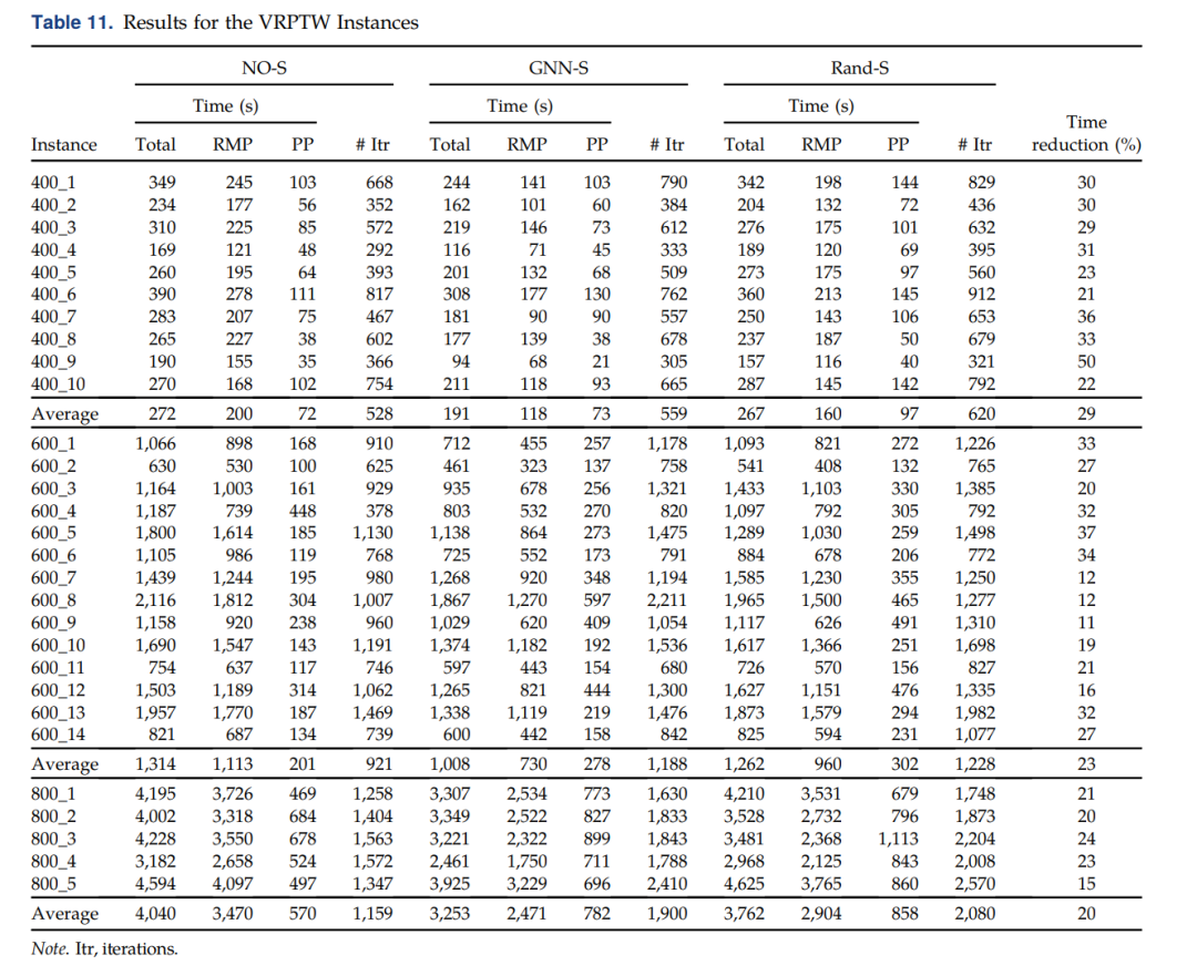
The last column corresponds to the time reduction when comparing GNN-S with NO-S. One can see that the column selection with the GNN model gives positive results, yielding average reductions ranging from 20%–29%. These reductions could have been larger if the number of CG iterations performed had not increased.