
Python圖像處理介紹--彩色圖像的直方圖處理
點擊上方“小白學視覺”,選擇加"星標"或“置頂”
重磅干貨,第一時間送達

引言
在昨天的文章中我們介紹了基于灰度圖像的直方圖處理,也簡單的提到了彩色圖像的直方圖處理,但是沒有討論最好的方法。
讓我們從導入所有需要的庫開始吧!
import numpy as npimport matplotlib.pyplot as pltfrom skimage.io import imread, imshowimport matplotlib.pyplot as pltfrom skimage.exposure import histogram, cumulative_distributionfrom scipy.stats import norm
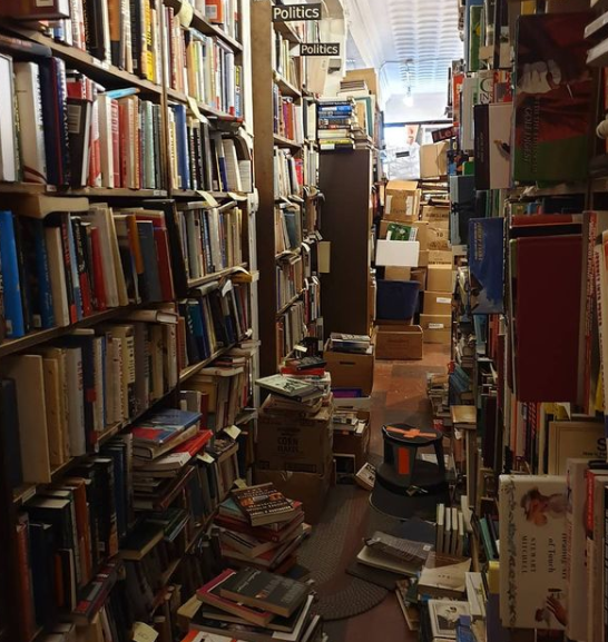
現(xiàn)在讓我們載入圖像。
dark_image = imread('dark_books.png');plt.figure(num=None, figsize=(8, 6), dpi=80)imshow(dark_image);
為了幫助我們更好地了解此圖像中的 RGB 圖層,讓我們隔離每個單獨的通道。
def rgb_splitter(image):rgb_list = ['Reds','Greens','Blues']fig, ax = plt.subplots(1, 3, figsize=(17,7), sharey = True)for i in range(3):ax[i].imshow(image[:,:,i], cmap = rgb_list[i])ax[i].set_title(rgb_list[i], fontsize = 22)ax[i].axis('off')fig.tight_layout()rgb_splitter(dark_image)
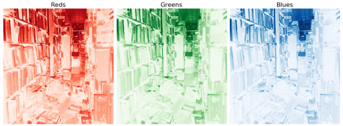
現(xiàn)在我們已經(jīng)對單個顏色通道有了大致的了解,現(xiàn)在查看它們的CDF。
def df_plotter(image):freq_bins = [cumulative_distribution(image[:,:,i]) for i inrange(3)]target_bins = np.arange(255)target_freq = np.linspace(0, 1, len(target_bins))names = ['Red', 'Green', 'Blue']line_color = ['red','green','blue']f_size = 20fig, ax = plt.subplots(1, 3, figsize=(17,5))for n, ax in enumerate(ax.flatten()):ax.set_title(f'{names[n]}', fontsize = f_size)ax.step(freq_bins[n][1], freq_bins[n][0], c=line_color[n],label='Actual CDF')ax.plot(target_bins,target_freq,c='gray',label='Target CDF',linestyle = '--')df_plotter(dark_image)
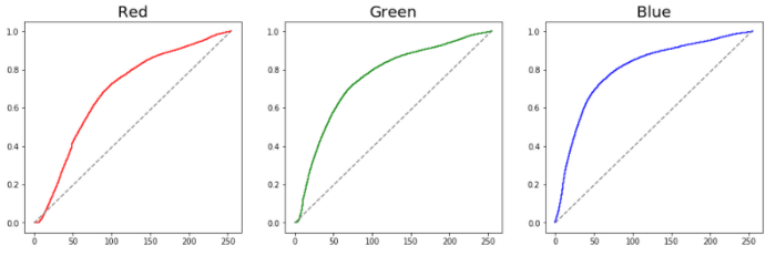
正如我們所看到的,這三個通道都離理想化的直線相當遠。為了解決這個問題,讓我們簡單地對其CDF進行插值。
def rgb_adjuster_lin(image):target_bins = np.arange(255)target_freq = np.linspace(0, 1, len(target_bins))freq_bins = [cumulative_distribution(image[:,:,i]) for i inrange(3)]names = ['Reds', 'Blues', 'Greens']line_color = ['red','green','blue']adjusted_figures = []f_size = 20fig, ax = plt.subplots(1,3, figsize=[15,5])for n, ax in enumerate(ax.flatten()):interpolation = np.interp(freq_bins[n][0], target_freq,target_bins)adjusted_image = img_as_ubyte(interpolation[image[:,:,n]].astype(int))ax.set_title(f'{names[n]}', fontsize = f_size)ax.imshow(adjusted_image, cmap = names[n])adjusted_figures.append([adjusted_image])fig.tight_layout()fig, ax = plt.subplots(1,3, figsize=[15,5])for n, ax in enumerate(ax.flatten()):interpolation = np.interp(freq_bins[n][0], target_freq,target_bins)adjusted_image = img_as_ubyte(interpolation[image[:,:,n]].astype(int))freq_adj, bins_adj = cumulative_distribution(adjusted_image)ax.set_title(f'{names[n]}', fontsize = f_size)ax.step(bins_adj, freq_adj, c=line_color[n], label='ActualCDF')ax.plot(target_bins,target_freq,c='gray',label='Target CDF',linestyle = '--')fig.tight_layout()return adjusted_figureschannel_figures = return adjusted_figures

我們看到每個顏色通道都有顯著改善。
此外,請注意上面的函數(shù)是如何將所有這些值作為列表返回。這將為我們的最后一步提供很好的幫助,將所有這些重新組合成一張圖片。為了讓我們更好地了解如何做到這一點,讓我們檢查一下我們的列表。
print(channel_figures)print(f'Total Inner Lists : {len(channel_figures)}')

我們看到在變量channel_figures中有三個列表。這些列表代表RGB通道的值。在下面,我們可以將所有這些值重新組合在一起。
plt.figure(num=None, figsize=(10, 8), dpi=80)imshow(np.dstack((channel_figures[0][0],channel_figures[1][0],channel_figures[2][0])));
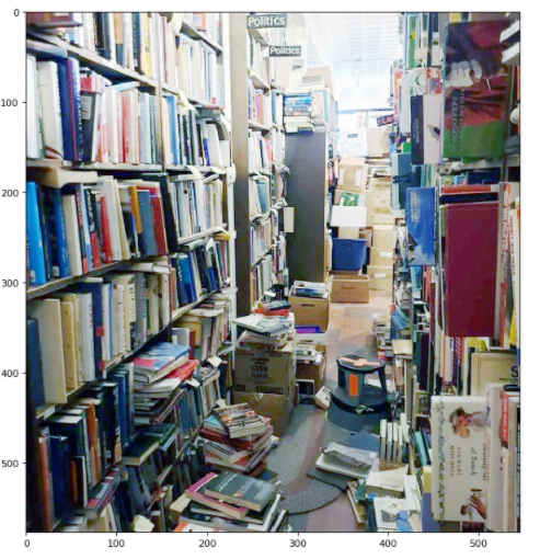
請注意圖像處理前后這種差異是多么顯著。圖像不僅明亮了許多,黃色的陰影也被移除了。讓我們在不同的圖像上進行同樣的處理試試。
dark_street = imread('dark_street.png');plt.figure(num=None, figsize=(8, 6), dpi=80)imshow(dark_street);

現(xiàn)在我們已經(jīng)加載了新的圖片,讓我們簡單地通過函數(shù)來處理。
channel_figures_street = adjusted_image_data = rgb_adjuster_lin(dark_street)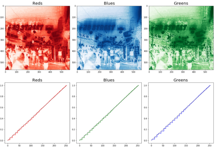
plt.figure(num=None, figsize=(10, 8), dpi=80)imshow(np.dstack((channel_figures_street [0][0],channel_figures_street [1][0],??????????????????channel_figures_street?[2][0])));
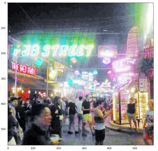
我們可以看到驚人的變化。不可否認,這張照片曝光有點過度。這可能是因為后面有明顯的霓虹燈。在以后的文章中,我們將學習如何微調我們的方法,以使我們的函數(shù)更加通用。
總結
在本文中,我們學習了如何調整每個RGB通道以保留圖像的顏色信息。這種技術是對以前的灰度調整方法的重大改進。
交流群
歡迎加入公眾號讀者群一起和同行交流,目前有SLAM、三維視覺、傳感器、自動駕駛、計算攝影、檢測、分割、識別、醫(yī)學影像、GAN、算法競賽等微信群(以后會逐漸細分),請掃描下面微信號加群,備注:”昵稱+學校/公司+研究方向“,例如:”張三?+?上海交大?+?視覺SLAM“。請按照格式備注,否則不予通過。添加成功后會根據(jù)研究方向邀請進入相關微信群。請勿在群內發(fā)送廣告,否則會請出群,謝謝理解~