
使用關(guān)鍵點進(jìn)行小目標(biāo)檢測
【GiantPandaCV導(dǎo)語】本文是筆者出于興趣搞了一個小的庫,主要是用于定位紅外小目標(biāo)。由于其具有尺度很小的特點,所以可以嘗試用點的方式代表其位置。本文主要采用了回歸和heatmap兩種方式來回歸關(guān)鍵點,是一個很簡單基礎(chǔ)的項目,代碼量很小,可供新手學(xué)習(xí)。
1. 數(shù)據(jù)來源
數(shù)據(jù)集:數(shù)據(jù)來源自小武,經(jīng)過小武的授權(quán)使用,但不會公開。本項目只用了其中很少一部分共108張圖片。
標(biāo)注工具:https://github.com/pprp/landmark_annotation
標(biāo)注工具也可以在GiantPandaCV公眾號后臺回復(fù)“l(fā)andmark”關(guān)鍵字獲取
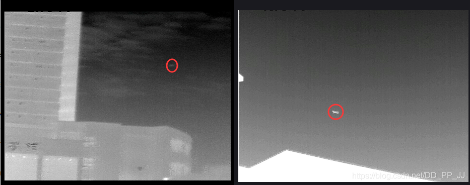
上圖是數(shù)據(jù)集中的兩張圖片,紅圈代表對應(yīng)的目標(biāo),標(biāo)注的時候只需要在其中心點一下即可得到該點對應(yīng)的橫縱坐標(biāo)。
該數(shù)據(jù)集有一個特點,每張圖只有一個目標(biāo)(不然沒法用簡單的方法回歸),多余一個目標(biāo)的圖片被剔除了。
1
0.42 0.596
以上是一個標(biāo)注文件的例子,1.jpg對應(yīng)1.txt
2. 回歸確定關(guān)鍵點
回歸確定關(guān)鍵點比較簡單,網(wǎng)絡(luò)部分采用手工構(gòu)建的一個兩層的小網(wǎng)絡(luò),訓(xùn)練采用的是MSELoss。
這部分代碼在:https://github.com/pprp/SimpleCVReproduction/tree/master/simple_keypoint/regression
2.1 數(shù)據(jù)加載
數(shù)據(jù)的組織比較簡單,按照以下格式組織:
- data
	- images
		- 1.jpg
		- 2.jpg
		- ...
	- labels
		- 1.txt
		- 2.txt
		- ...
重寫一下Dataset類,用于加載數(shù)據(jù)集。
class KeyPointDatasets(Dataset):
    def __init__(self, root_dir="./data", transforms=None):
        super(KeyPointDatasets, self).__init__()
        self.img_path = os.path.join(root_dir, "images")
        # self.txt_path = os.path.join(root_dir, "labels")

        self.img_list = glob.glob(os.path.join(self.img_path, "*.jpg"))
        self.txt_list = [item.replace(".jpg", ".txt").replace(
            "images", "labels") for item in self.img_list]

        if transforms is not None:
            self.transforms = transforms

    def __getitem__(self, index):
        img = self.img_list[index]
        txt = self.txt_list[index]

        img = cv2.imread(img)

        if self.transforms:
            img = self.transforms(img)

        label = []

        with open(txt, "r") as f:
            for i, line in enumerate(f):
                if i == 0:
                    # 第一行
                    num_point = int(line.strip())
                else:
                    x1, y1 = [(t.strip()) for t in line.split()]
                    # range from 0 to 1
                    x1, y1 = float(x1), float(y1)

                    tmp_label = (x1, y1)
                    label.append(tmp_label)

        return img, torch.tensor(label[0])

    def __len__(self):
        return len(self.img_list)

    @staticmethod
    def collect_fn(batch):
        imgs, labels = zip(*batch)
        return torch.stack(imgs, 0), torch.stack(labels, 0)
返回的結(jié)果是圖片和對應(yīng)坐標(biāo)位置。
2.2 網(wǎng)絡(luò)模型
import torch
import torch.nn as nn

class KeyPointModel(nn.Module):
    def __init__(self):
        super(KeyPointModel, self).__init__()
        self.conv1 = nn.Conv2d(3, 6, 3, 1, 1)
        self.bn1 = nn.BatchNorm2d(6)
        self.relu1 = nn.ReLU(True)
        self.maxpool1 = nn.MaxPool2d((2, 2))

        self.conv2 = nn.Conv2d(6, 12, 3, 1, 1)
        self.bn2 = nn.BatchNorm2d(12)
        self.relu2 = nn.ReLU(True)
        self.maxpool2 = nn.MaxPool2d((2, 2))

        self.gap = nn.AdaptiveMaxPool2d(1)
        self.classifier = nn.Sequential(
            nn.Linear(12, 2),
            nn.Sigmoid()
        )

    def forward(self, x):
        x = self.conv1(x)
        x = self.bn1(x)
        x = self.relu1(x)
        x = self.maxpool1(x)

        x = self.conv2(x)
        x = self.bn2(x)
        x = self.relu2(x)
        x = self.maxpool2(x)

        x = self.gap(x)
        x = x.view(x.shape[0], -1)
        return self.classifier(x)
其結(jié)構(gòu)就是卷積+pooling+卷積+pooling+global average pooling+Linear,返回長度為2的tensor。
2.3 訓(xùn)練
def train(model, epoch, dataloader, optimizer, criterion):
    model.train()
    for itr, (image, label) in enumerate(dataloader):
        bs = image.shape[0]
        output = model(image)
        loss = criterion(output, label)

        optimizer.zero_grad()
        loss.backward()
        optimizer.step()

        if itr % 4 == 0:
            print("epoch:%2d|step:%04d|loss:%.6f" % (epoch, itr, loss.item()/bs))
            vis.plot_many_stack({"train_loss": loss.item()*100/bs})

total_epoch = 300
bs = 10
########################################
transforms_all = transforms.Compose([
    transforms.ToPILImage(),
    transforms.Resize((360,480)),
    transforms.ToTensor(),
    transforms.Normalize(mean=[0.4372, 0.4372, 0.4373],
                         std=[0.2479, 0.2475, 0.2485])
])

datasets = KeyPointDatasets(root_dir="./data", transforms=transforms_all)

data_loader = DataLoader(datasets, shuffle=True,
                         batch_size=bs, collate_fn=datasets.collect_fn)

model = KeyPointModel()

optimizer = torch.optim.Adam(model.parameters(), lr=3e-4)
# criterion = torch.nn.SmoothL1Loss()
criterion = torch.nn.MSELoss()
scheduler = torch.optim.lr_scheduler.StepLR(optimizer,
                                            step_size=30,
                                            gamma=0.1)

for epoch in range(total_epoch):
    train(model, epoch, data_loader, optimizer, criterion)
    loss = test(model, epoch, data_loader, criterion)

    if epoch % 10 == 0:
        torch.save(model.state_dict(),
                   "weights/epoch_%d_%.3f.pt" % (epoch, loss*1000))
loss部分使用Smooth L1 loss或者M(jìn)SE loss均可。
MSE Loss:
Smooth L1 Loss:
2.4 測試結(jié)果
3. heatmap確定關(guān)鍵點
這部分代碼很多參考了CenterNet,不過曾經(jīng)嘗試CenterNet中的loss在這個問題上收斂效果不好,所以參考了kaggle人臉關(guān)鍵點定位的解決方法,發(fā)現(xiàn)使用簡單的MSELoss效果就很好。
3.1 數(shù)據(jù)加載
這部分和CenterNet構(gòu)建heatmap的過程類似,不過半徑的確定是人工的。因為數(shù)據(jù)集中的目標(biāo)都比較小,半徑的范圍最大不超過半徑為30個像素的圓。
class KeyPointDatasets(Dataset):
    def __init__(self, root_dir="./data", transforms=None):
        super(KeyPointDatasets, self).__init__()

        self.down_ratio = 1
        self.img_w = 480 // self.down_ratio
        self.img_h = 360 // self.down_ratio

        self.img_path = os.path.join(root_dir, "images")

        self.img_list = glob.glob(os.path.join(self.img_path, "*.jpg"))
        self.txt_list = [item.replace(".jpg", ".txt").replace(
            "images", "labels") for item in self.img_list]

        if transforms is not None:
            self.transforms = transforms

    def __getitem__(self, index):
        img = self.img_list[index]
        txt = self.txt_list[index]

        img = cv2.imread(img)

        if self.transforms:
            img = self.transforms(img)

        label = []

        with open(txt, "r") as f:
            for i, line in enumerate(f):
                if i == 0:
                    # 第一行
                    num_point = int(line.strip())
                else:
                    x1, y1 = [(t.strip()) for t in line.split()]
                    # range from 0 to 1
                    x1, y1 = float(x1), float(y1)
                    cx, cy = x1 * self.img_w, y1 * self.img_h
                    heatmap = np.zeros((self.img_h, self.img_w))
                    draw_umich_gaussian(heatmap, (cx, cy), 30)
        return img, torch.tensor(heatmap).unsqueeze(0)

    def __len__(self):
        return len(self.img_list)

    @staticmethod
    def collect_fn(batch):
        imgs, labels = zip(*batch)
        return torch.stack(imgs, 0), torch.stack(labels, 0)
核心函數(shù)是draw_umich_gaussian,具體如下:
def gaussian2D(shape, sigma=1):
    m, n = [(ss - 1.) / 2. for ss in shape]
    y, x = np.ogrid[-m:m + 1, -n:n + 1]
    h = np.exp(-(x * x + y * y) / (2 * sigma * sigma))
    h[h < np.finfo(h.dtype).eps * h.max()] = 0
    # 限制最小的值
    return h

def draw_umich_gaussian(heatmap, center, radius, k=1):
    diameter = 2 * radius + 1
    gaussian = gaussian2D((diameter, diameter), sigma=diameter / 6)
    # 一個圓對應(yīng)內(nèi)切正方形的高斯分布
    x, y = int(center[0]), int(center[1])
    width, height = heatmap.shape
    left, right = min(x, radius), min(width - x, radius + 1)
    top, bottom = min(y, radius), min(height - y, radius + 1)
    masked_heatmap = heatmap[y - top:y + bottom, x - left:x + right]
    masked_gaussian = gaussian[radius - top:radius +
                               bottom, radius - left:radius + right]
    if min(masked_gaussian.shape) > 0 and min(masked_heatmap.shape) > 0:  # TODO debug
        np.maximum(masked_heatmap, masked_gaussian * k, out=masked_heatmap)
        # 將高斯分布覆蓋到heatmap上,取最大,而不是疊加
    return heatmap
sigma參數(shù)直接沿用了CenterNet中的設(shè)置,沒有調(diào)節(jié)這個超參數(shù)。
3.2 網(wǎng)絡(luò)結(jié)構(gòu)
網(wǎng)絡(luò)結(jié)構(gòu)參考了知乎上一個復(fù)現(xiàn)YOLOv3中提到的模塊,Sematic Embbed Block(SEB)用于上采樣部分,將來自低分辨率的特征圖進(jìn)行上采樣,然后使用3x3卷積和1x1卷積統(tǒng)一通道個數(shù),最后將低分辨率特征圖和高分辨率特征圖相乘得到融合結(jié)果。
class SematicEmbbedBlock(nn.Module):
    def __init__(self, high_in_plane, low_in_plane, out_plane):
        super(SematicEmbbedBlock, self).__init__()
        self.conv3x3 = nn.Conv2d(high_in_plane, out_plane, 3, 1, 1)
        self.upsample = nn.UpsamplingBilinear2d(scale_factor=2)

        self.conv1x1 = nn.Conv2d(low_in_plane, out_plane, 1)

    def forward(self, high_x, low_x):
        high_x = self.upsample(self.conv3x3(high_x))
        low_x = self.conv1x1(low_x)
        return high_x * low_x


class KeyPointModel(nn.Module):
    """
    downsample ratio=2
    """

    def __init__(self):
        super(KeyPointModel, self).__init__()
        self.conv1 = nn.Conv2d(3, 6, 3, 1, 1)
        self.bn1 = nn.BatchNorm2d(6)
        self.relu1 = nn.ReLU(True)
        self.maxpool1 = nn.MaxPool2d((2, 2))

        self.conv2 = nn.Conv2d(6, 12, 3, 1, 1)
        self.bn2 = nn.BatchNorm2d(12)
        self.relu2 = nn.ReLU(True)
        self.maxpool2 = nn.MaxPool2d((2, 2))

        self.conv3 = nn.Conv2d(12, 20, 3, 1, 1)
        self.bn3 = nn.BatchNorm2d(20)
        self.relu3 = nn.ReLU(True)
        self.maxpool3 = nn.MaxPool2d((2, 2))

        self.conv4 = nn.Conv2d(20, 40, 3, 1, 1)
        self.bn4 = nn.BatchNorm2d(40)
        self.relu4 = nn.ReLU(True)

        self.seb1 = SematicEmbbedBlock(40, 20, 20)
        self.seb2 = SematicEmbbedBlock(20, 12, 12)
        self.seb3 = SematicEmbbedBlock(12, 6, 6)

        self.heatmap = nn.Conv2d(6, 1, 1)

    def forward(self, x):
        x1 = self.conv1(x)
        x1 = self.bn1(x1)
        x1 = self.relu1(x1)

        m1 = self.maxpool1(x1)

        x2 = self.conv2(m1)
        x2 = self.bn2(x2)
        x2 = self.relu2(x2)

        m2 = self.maxpool2(x2)

        x3 = self.conv3(m2)
        x3 = self.bn3(x3)
        x3 = self.relu3(x3)

        m3 = self.maxpool3(x3)

        x4 = self.conv4(m3)
        x4 = self.bn4(x4)
        x4 = self.relu4(x4)

        up1 = self.seb1(x4, x3)
        up2 = self.seb2(up1, x2)
        up3 = self.seb3(up2, x1)

        out = self.heatmap(up3)
        return out
網(wǎng)絡(luò)模型也是自己寫的小網(wǎng)絡(luò),用了四個卷積層,三個池化層,然后進(jìn)行了三次上采樣。最終輸出分辨率和輸入分辨率相同。
3.3 訓(xùn)練過程
訓(xùn)練過程和基于回歸的方法幾乎一樣,代碼如下:
datasets = KeyPointDatasets(root_dir="./data", transforms=transforms_all)

data_loader = DataLoader(datasets, shuffle=True,
                         batch_size=bs, collate_fn=datasets.collect_fn)

model = KeyPointModel()

if torch.cuda.is_available():
    model = model.cuda()

optimizer = torch.optim.Adam(model.parameters(), lr=3e-3)
criterion = torch.nn.MSELoss()  # compute_loss
scheduler = torch.optim.lr_scheduler.StepLR(optimizer,
                                                step_size=30,
                                                gamma=0.1)

for epoch in range(total_epoch):
    train(model, epoch, data_loader, optimizer, criterion, scheduler)
    loss = test(model, epoch, data_loader, criterion)

    if epoch % 5 == 0:
        torch.save(model.state_dict(),
                   "weights/epoch_%d_%.3f.pt" % (epoch, loss*10000))
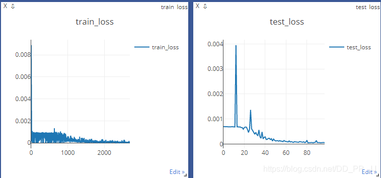
用的是MSELoss進(jìn)行監(jiān)督,訓(xùn)練曲線如下:
3.4 測試過程
測試過程和CenterNet的推理過程一致,也用到了3x3的maxpooling來篩選極大值點
for iter, (image, label) in enumerate(dataloader):
# print(image.shape)
bs = image.shape[0]
hm = model(image)
hm = _nms(hm)
hm = hm.detach().numpy()
for i in range(bs):
hm = hm[i]
hm = np.maximum(hm, 0)
hm = hm/np.max(hm)
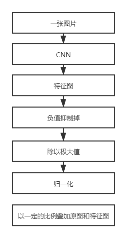
hm = normalization(hm)
hm = np.uint8(255 * hm)
hm = hm[0]
# heatmap = torch.sigmoid(heatmap)
# hm = cv2.cvtColor(hm, cv2.COLOR_RGB2BGR)
hm = cv2.applyColorMap(hm, cv2.COLORMAP_JET)
cv2.imwrite("./test_output/output_%d_%d.jpg" % (iter, i), hm)
cv2.waitKey(0)
以上的nms和topk代碼都在CenterNet系列最后一篇講過了。這里直接對模型輸出結(jié)果使用nms,然后進(jìn)行可視化,結(jié)果如下:
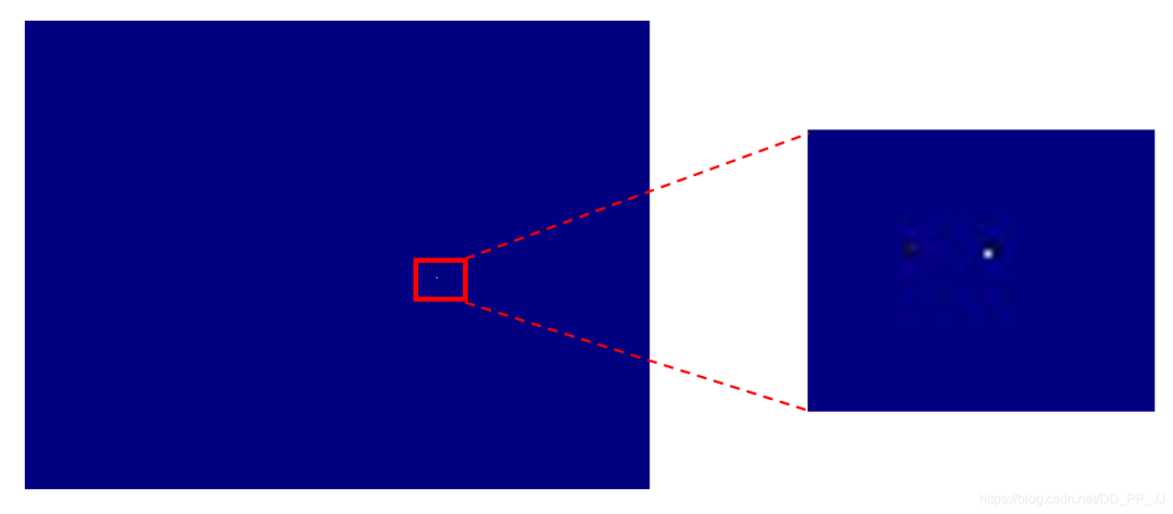
上圖中白色的點就是目標(biāo)位置,為了更形象的查看結(jié)果,detect.py部分負(fù)責(zé)可視化。
3.5 可視化
可視化的問題經(jīng)常遇見,比如CAM、Grad CAM等可視化特征圖的時候就會碰到。以下是可視化的一個簡單的方法(參考了CSDN的一位博主的方案,具體鏈接因太過久遠(yuǎn)找不到了)。
具體實現(xiàn)代碼如下:
def normalization(data):
    _range = np.max(data) - np.min(data)
    return (data - np.min(data)) / _range

heatmap = model(img_tensor_list)
heatmap = heatmap.squeeze().cpu()

for i in range(bs):
    img_path = img_list[i]
    img = cv2.imread(img_path)
    img = cv2.resize(img, (480, 360))
    single_map = heatmap[i]
    hm = single_map.detach().numpy()
    hm = np.maximum(hm, 0)
    hm = hm/np.max(hm)
    hm = normalization(hm)
    hm = np.uint8(255 * hm)
    hm = cv2.applyColorMap(hm, cv2.COLORMAP_JET)
    hm = cv2.resize(hm, (480, 360))
    superimposed_img = hm * 0.2 + img
    coord_x, coord_y = landmark_coord[i]
    cv2.circle(superimposed_img, (int(coord_x), int(coord_y)), 2, (0, 0, 0), thickness=-1)
    cv2.imwrite("./output2/%s_out.jpg" % (img_name_list[i]), superimposed_img)
注意通過處理以后的hm和原圖疊加的時候0.2只是一個參考值,這個值既不會影響原圖顯示又能將heatmap中重點關(guān)注的位置可視化出來。
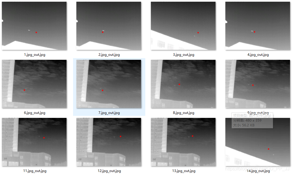
結(jié)果如下:
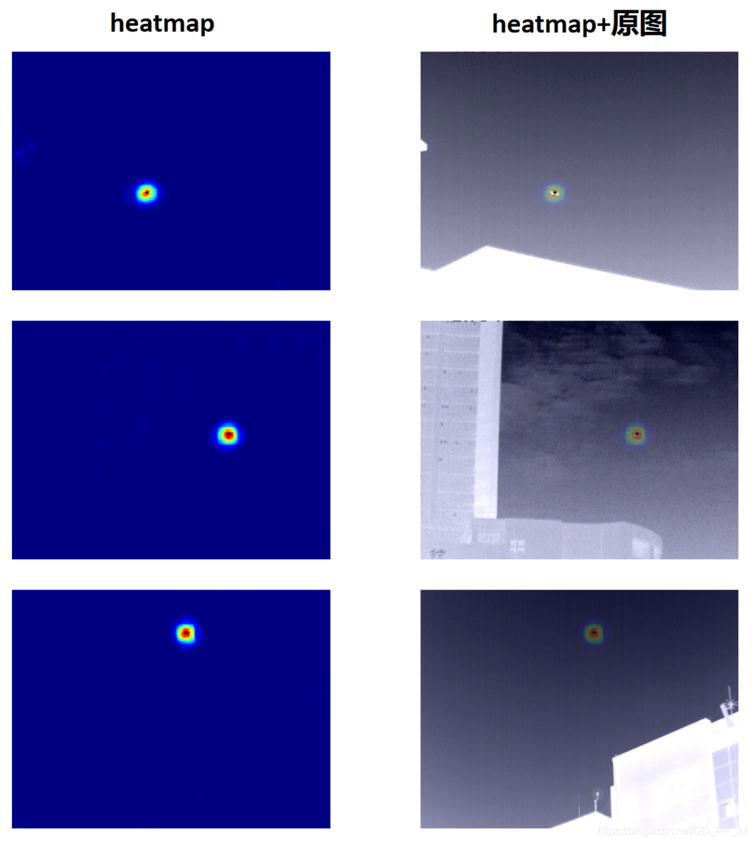
可以看到,定位結(jié)果要比回歸更準(zhǔn)一些,圖中黑色點是獲取到最終坐標(biāo)的位置,幾乎和目標(biāo)是重疊的狀態(tài),效果比較理想。
4. 總結(jié)
筆者做這個小項目初心是想搞清楚如何用關(guān)鍵點進(jìn)行定位的,關(guān)鍵點被用在很多領(lǐng)域比如人臉關(guān)鍵點定位、車牌定位、人體姿態(tài)檢測、目標(biāo)檢測等等領(lǐng)域。當(dāng)時用小武的數(shù)據(jù)的時候,發(fā)現(xiàn)這個數(shù)據(jù)集的特點就是目標(biāo)很小,比較適合用關(guān)鍵點來做。之后又開始陸陸續(xù)續(xù)看CenterNet源碼,借鑒了其中很多代碼,這才完成了這個小項目。
由于本人水平有限,可能使用heatmap進(jìn)行關(guān)鍵點定位的方式有些地方并不合理,是東拼西湊而成的,如果有建議可以在下方添加筆者微信。
為了感謝讀者朋友們的長期支持,我們今天將送出3本由中國工信出版社和人民郵電出版社提供的《深度學(xué)習(xí)訓(xùn)練營》書籍,對本書感興趣的可以在留言版留言,我們將抽取其中三位讀者送出一本正版書籍。
沒中獎的讀者如果有對此書感興趣的,可以考慮點擊下方的當(dāng)當(dāng)網(wǎng)鏈接自行購買。
對文章有疑問或者想加入交流群,歡迎添加筆者微信
為了方便各位獲取公眾號獲取資料,可以加入QQ群獲取資源,更歡迎分享資源