【機(jī)器學(xué)習(xí)】快速入門簡單線性回歸 (SLR)

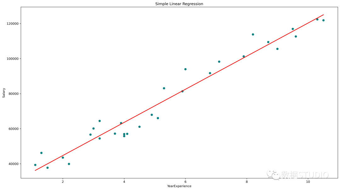
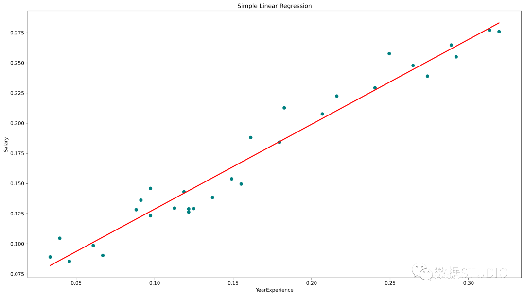
簡單線性回歸圖（青色散點(diǎn)為實(shí)際值，紅線為預(yù)測值）

statsmodels.api、statsmodels.formula.api 和 scikit-learn 的 Python 中的 SLR

今天云朵君將和大家一起學(xué)習(xí)回歸算法的基礎(chǔ)知識。并取一個樣本數(shù)據(jù)集，進(jìn)行探索性數(shù)據(jù)分析(EDA)并使用 statsmodels.api、statsmodels.formula.api 和 scikit-learn 實(shí)現(xiàn) 簡單線性回歸(SLR)。

什么是回歸算法

回歸是一種用于預(yù)測連續(xù)特征的"監(jiān)督機(jī)器學(xué)習(xí)"算法。

線性回歸是最簡單的回歸算法，它試圖通過將線性方程/最佳擬合線擬合到觀察數(shù)據(jù)，來模擬因變量與一個或多個自變量之間的關(guān)系。

根據(jù)輸入特征的數(shù)量，線性回歸可以有兩種類型：

• 簡單線性回歸 (SLR)
• 多元線性回歸 (MLR)

在簡單線性回歸 (SLR) 中，根據(jù)單一的輸入變量預(yù)測輸出變量。在多元線性回歸 (MLR) 中，根據(jù)多個輸入變量預(yù)測輸出。

輸入變量也可以稱為獨(dú)立/預(yù)測變量，輸出變量稱為因變量。

SLR 的方程為，其中， 是因變量， 是預(yù)測變量， 是模型的系數(shù)/參數(shù)，Epsilon(?) 是一個稱為誤差項(xiàng)的隨機(jī)變量。

普通最小二乘法(OLS)和梯度下降是兩種常見的算法，用于為最小平方誤差總和找到正確的系數(shù)。

如何實(shí)現(xiàn)回歸算法

目標(biāo)：建立一個簡單的線性回歸模型，使用多年的經(jīng)驗(yàn)來預(yù)測加薪。

首先導(dǎo)入必要的庫

這里必要的庫是 Pandas、用于處理數(shù)據(jù)框的 NumPy、用于可視化的 matplotlib、seaborn，以及用于構(gòu)建回歸模型的 sklearn、statsmodels。

import?pandas?as?pd?
import?numpy?as?np
import?matplotlib.pyplot?as?plt
%matplotlib?inline
import?seaborn?as?sns
from?scipy?import?stats
from?scipy.stats?import?probplot
import?statsmodels.api?as?sm?
import?statsmodels.formula.api?as?smf?
from?sklearn?import?preprocessing
from?sklearn.linear_model?import?LinearRegression
from?sklearn.model_selection?import?train_test_split
from?sklearn.metrics?import?mean_squared_error,?r2_score

從 CSV 文件創(chuàng)建 Pandas 數(shù)據(jù)框。數(shù)據(jù)獲取：在公眾號『數(shù)據(jù)STUDIO』后臺聯(lián)系云朵君獲取！

df?=?pd.read_csv("Salary_Data.csv")

探索性數(shù)據(jù)分析(EDA)

EDA的基本步驟

• 了解數(shù)據(jù)集

1. 確定數(shù)據(jù)集的大小
2. 確定特征的數(shù)量
3. 識別特征及特征的數(shù)據(jù)類型
4. 檢查數(shù)據(jù)集是否有缺失值、異常值
5. 通過特征的缺失值、異常值的數(shù)量

• 處理缺失值和異常值
• 編碼分類變量
• 圖形單變量分析，雙變量
• 規(guī)范化和縮放

df.info()

RangeIndex: 30 entries, 0 to 29
Data columns (total 2 columns):
 #   Column           Non-Null Count  Dtype  
---  ------           --------------  -----  
 0   YearsExperience  30 non-null     float64
 1   Salary           30 non-null     float64
dtypes: float64(2)
memory usage: 608.0 bytes

len(df.columns)?#?確定特征的數(shù)量
df.columns?#?識別特征

df.shape?#?確定數(shù)據(jù)集的大小
df.dtypes?#?確定特性的數(shù)據(jù)類型
df.isnull().values.any()?#?檢查數(shù)據(jù)集是否有缺失值
df.isnull().sum()?#?檢查數(shù)據(jù)集是否有缺失值

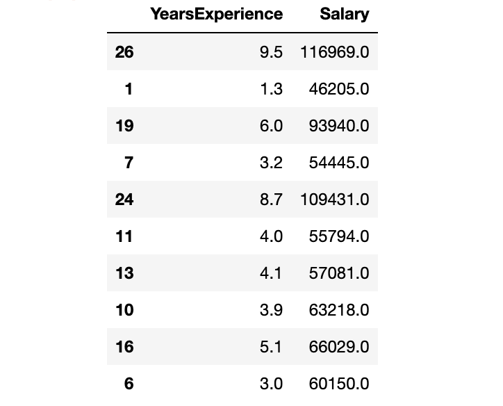
數(shù)據(jù)集有兩列：YearsExperience、Salary。并且兩者都是浮點(diǎn)數(shù)據(jù)類型。數(shù)據(jù)集中有 30 條記錄，沒有空值或異常值。

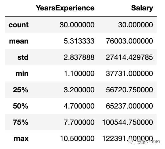
描述性統(tǒng)計(jì)包括那些總結(jié)數(shù)據(jù)集分布的集中趨勢、分散和形狀的統(tǒng)計(jì)，不包括NaN值

df.describe()?

圖形單變量分析

對于單變量分析，可以使用直方圖、密度圖、箱線圖或小提琴圖，以及正態(tài) QQ 圖來幫助我們了解數(shù)據(jù)點(diǎn)的分布和異常值的存在。

小提琴圖是一種繪制數(shù)字?jǐn)?shù)據(jù)的方法。它類似于箱線圖，但在每一側(cè)都添加了一個旋轉(zhuǎn)的核密度圖。

Python代碼：

#?Histogram
#?We?can?use?either?plt.hist?or?sns.histplot
plt.figure(figsize=(20,10))
plt.subplot(2,4,1)
plt.hist(df['YearsExperience'],?density=False)
plt.title("Histogram?of?'YearsExperience'")
plt.subplot(2,4,5)
plt.hist(df['Salary'],?density=False)
plt.title("Histogram?of?'Salary'")

#?Density?plot
plt.subplot(2,4,2)
sns.distplot(df['YearsExperience'],?kde=True)
plt.title("Density?distribution?of?'YearsExperience'")
plt.subplot(2,4,6)
sns.distplot(df['Salary'],?kde=True)
plt.title("Density?distribution?of?'Salary'")

#?boxplot?or?violin?plot
#?小提琴圖是一種繪制數(shù)字?jǐn)?shù)據(jù)的方法。
#?它類似于箱形圖，在每一邊添加了一個旋轉(zhuǎn)的核密度圖
plt.subplot(2,4,3)
#?plt.boxplot(df['YearsExperience'])
sns.violinplot(df['YearsExperience'])
#?plt.title("Boxlpot?of?'YearsExperience'")
plt.title("Violin?plot?of?'YearsExperience'")
plt.subplot(2,4,7)
#?plt.boxplot(df['Salary'])
sns.violinplot(df['Salary'])
#?plt.title("Boxlpot?of?'Salary'")
plt.title("Violin?plot?of?'Salary'")

#?Normal?Q-Q?plot
plt.subplot(2,4,4)
probplot(df['YearsExperience'],?plot=plt)
plt.title("Q-Q?plot?of?'YearsExperience'")
plt.subplot(2,4,8)
probplot(df['Salary'],?plot=plt)
plt.title("Q-Q?plot?of?'Salary'")

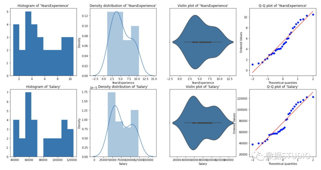
從上面的圖形表示，我們可以說我們的數(shù)據(jù)中沒有異常值，并且 YearsExperience looks like normally distributed, and Salary doesn't look normal。我們可以使用Shapiro Test。

Python代碼：

#?定義一個函數(shù)進(jìn)行?Shapiro?test

#?定義零備擇假設(shè)
Ho?=?'Data?is?Normal'
Ha?=?'Data?is?not?Normal'

#?定義重要度值
alpha?=?0.05
def?normality_check(df):
????for?columnName,?columnData?in?df.iteritems():
????????print("Shapiro?test?for?{columnName}".format(columnName=columnName))
????????res?=?stats.shapiro(columnData)
????#?print(res)
????????pValue?=?round(res[1],?2)
????????
????????#?Writing?condition
????????if?pValue?>?alpha:
????????????print("pvalue?=?{pValue}?>?{alpha}.?不能拒絕零假設(shè).?{Ho}".format(pValue=pValue,?alpha=alpha,?Ho=Ho))
????????else:
????????????print("pvalue?=?{pValue}?<=?{alpha}.?拒絕零假設(shè).?{Ha}".format(pValue=pValue,?alpha=alpha,?Ha=Ha))

#?Drive?code
normality_check(df)

Shapiro test for YearsExperience
pvalue = 0.1 > 0.05. 
不能拒絕零假設(shè). Data is Normal
Shapiro test for Salary
pvalue = 0.02 <= 0.05. 
拒絕零假設(shè). Data is not Normal

YearsExperience 是正態(tài)分布的，Salary 不是正態(tài)分布的。

雙變量可視化

對于數(shù)值與數(shù)值數(shù)據(jù)，我們繪制：散點(diǎn)圖、線圖、相關(guān)性熱圖、聯(lián)合圖來進(jìn)行數(shù)據(jù)探索。

Python 代碼：

#?Scatterplot?&?Line?plots
plt.figure(figsize=(20,10))
plt.subplot(1,3,1)
sns.scatterplot(data=df,?x="YearsExperience",?
????????????????y="Salary",?hue="YearsExperience",
????????????????alpha=0.6)
plt.title("Scatter?plot")
plt.subplot(1,3,2)
sns.lineplot(data=df,?x="YearsExperience",?y="Salary")
plt.title("Line?plot?of?YearsExperience,?Salary")
plt.subplot(1,3,3)
sns.lineplot(data=df)
plt.title('Line?Plot')

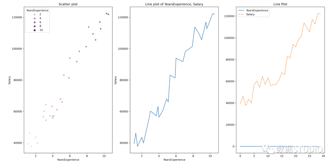
散點(diǎn)圖和線圖

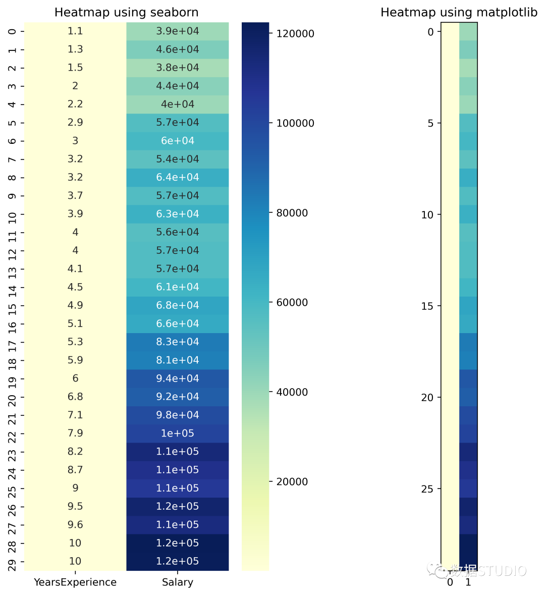
#?heatmap
plt.figure(figsize=(10,?10))
plt.subplot(1,?2,?1)
sns.heatmap(data=df,?cmap="YlGnBu",?annot?=?True)
plt.title("Heatmap?using?seaborn")
plt.subplot(1,?2,?2)
plt.imshow(df,?cmap?="YlGnBu")
plt.title("Heatmap?using?matplotlib")

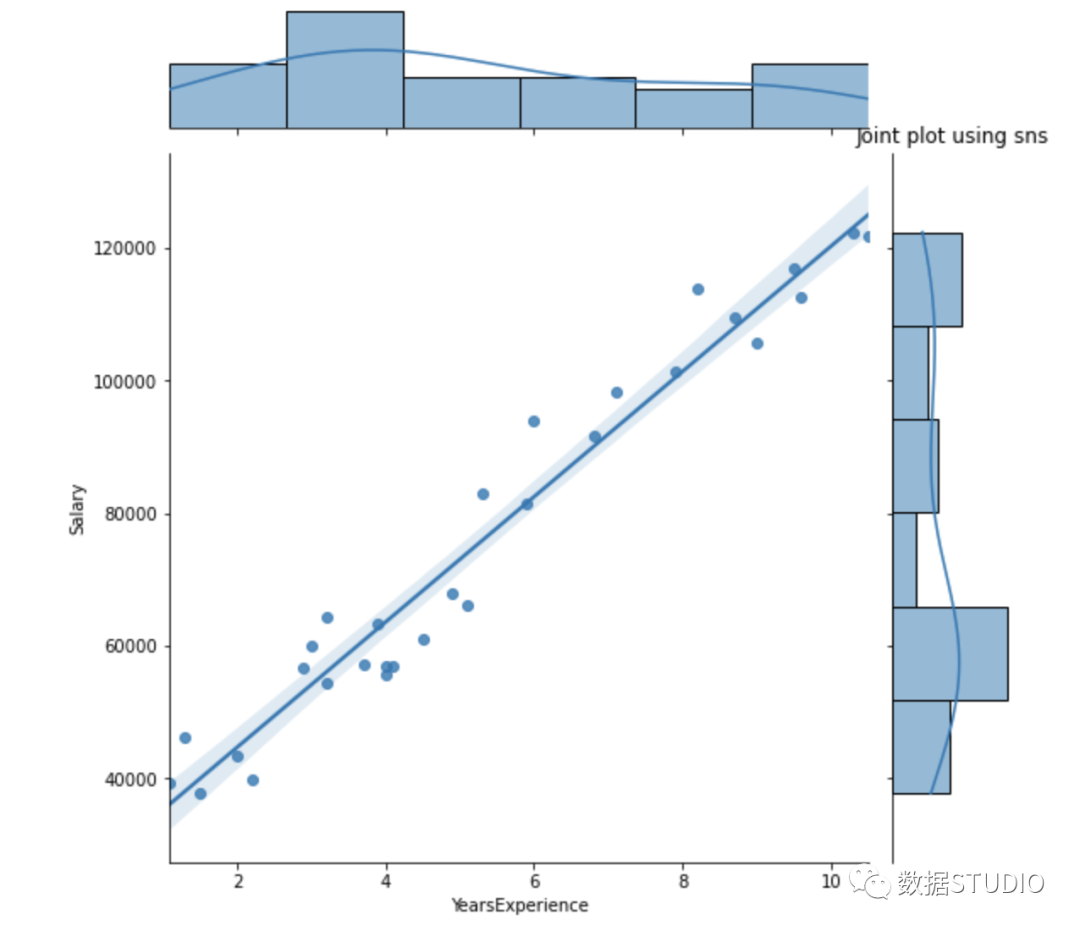
#?Joint?plot
sns.jointplot(x?=?"YearsExperience",?y?=?"Salary",?kind?=?"reg",?data?=?df)
plt.title("Joint?plot?using?sns")
#?類型可以是hex, kde, scatter, reg, hist。當(dāng)kind='reg'時，它顯示最佳擬合線。

使用 df.corr() 檢查變量之間是否存在相關(guān)性。

print("Correlation:?"+?'n',?df.corr())?
#?0.978，高度正相關(guān)
#?繪制相關(guān)矩陣的熱圖
plt.subplot(1,1,1)
sns.heatmap(df.corr(),?annot=True)

Correlation: 
                  YearsExperience    Salary
YearsExperience         1.000000  0.978242
Salary                  0.978242  1.000000

相關(guān)性=0.98，這是一個高正相關(guān)性。這意味著因變量隨著自變量的增加而增加。

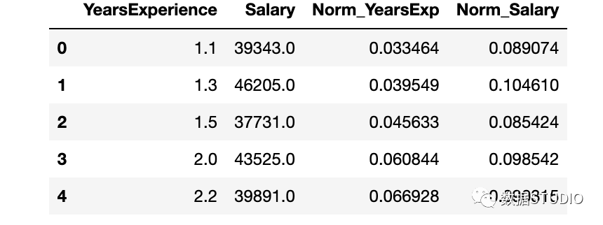
數(shù)據(jù)標(biāo)準(zhǔn)化

YearsExperience 和 Salary 列的值之間存在巨大差異。可以使用Normalization更改數(shù)據(jù)集中數(shù)字列的值以使用通用比例，而不會扭曲值范圍的差異或丟失信息。

我們使用sklearn.preprocessing.Normalize用來規(guī)范化我們的數(shù)據(jù)。它返回 0 到 1 之間的值。

#?創(chuàng)建新列來存儲規(guī)范化值
df['Norm_YearsExp']?=?preprocessing.normalize(df[['YearsExperience']],?axis=0)
df['Norm_Salary']?=?preprocessing.normalize(df[['Salary']],?axis=0)
df.head()

使用 sklearn 進(jìn)行線性回歸

LinearRegression() 擬合一個系數(shù)為的線性模型，以最小化數(shù)據(jù)集中觀察到的目標(biāo)與線性近似預(yù)測的目標(biāo)之間的殘差平方和。

def?regression(df):
??#?定義獨(dú)立和依賴的特性
????x?=?df.iloc[:,?1:2]
????y?=?df.iloc[:,?0:1]?
????#?print(x,y)

????#?實(shí)例化線性回歸對象
????regressor?=?LinearRegression()
????
????#?訓(xùn)練模型
????regressor.fit(x,y)

????#?檢查每個預(yù)測模型的系數(shù)
????print('n'+"Coeff?of?the?predictor:?",regressor.coef_)
????
????#?檢查截距項(xiàng)
????print("Intercept:?",regressor.intercept_)

????#?預(yù)測輸出值
????y_pred?=?regressor.predict(x)
#?????print(y_pred)

????#?檢查?MSE
????print("Mean?squared?error(MSE):?%.2f"?%?mean_squared_error(y,?y_pred))
????#?Checking?the?R2?value
????print("Coefficient?of?determination:?%.3f"?%?r2_score(y,?y_pred))?
??#?評估模型的性能，表示大部分?jǐn)?shù)據(jù)點(diǎn)落在最佳擬合線上
????
????#?可視化結(jié)果
????plt.figure(figsize=(18,?10))
????#?輸入和輸出值的散點(diǎn)圖
????plt.scatter(x,?y,?color='teal')
????#?輸入和預(yù)測輸出值的繪圖
????plt.plot(x,?regressor.predict(x),?color='Red',?linewidth=2?)
????plt.title('Simple?Linear?Regression')
????plt.xlabel('YearExperience')
????plt.ylabel('Salary')
??????
#?Driver?code
regression(df[['Salary',?'YearsExperience']])?#?0.957?accuracy
regression(df[['Norm_Salary',?'Norm_YearsExp']])?#?0.957?accuracy

Coeff of the predictor:  [[9449.96232146]]
Intercept:  [25792.20019867]
Mean squared error(MSE): 31270951.72
Coefficient of determination: 0.957

Coeff of the predictor:  [[0.70327706]]
Intercept:  [0.05839456]
Mean squared error(MSE): 0.00
Coefficient of determination: 0.957

使用 scikit-learn 中線性回歸模型實(shí)現(xiàn)了 95.7% 的準(zhǔn)確率，但在深入了解該模型中特征的相關(guān)性方面并沒有太多空間。接下來使用 statsmodels.api, statsmodels.formula.api 構(gòu)建一個模型。

使用 smf 的線性回歸

statsmodels.formula.api 中的預(yù)測變量必須單獨(dú)枚舉。該方法中，一個常量會自動添加到數(shù)據(jù)中。

def?smf_ols(df):
????#?定義獨(dú)立和依賴的特性
????x?=?df.iloc[:,?1:2]
????y?=?df.iloc[:,?0:1]?
#?????print(x)
????#?訓(xùn)練模型
????model?=?smf.ols('y~x',?data=df).fit()
????#?print?model?summary
????print(model.summary())
????
????#?預(yù)測?y
????y_pred?=?model.predict(x)
#?????print(type(y),?type(y_pred))
#?????print(y,?y_pred)

????y_lst?=?y.Salary.values.tolist()
#?????y_lst?=?y.iloc[:,?-1:].values.tolist()
????y_pred_lst?=?y_pred.tolist()????
#?????print(y_lst)
????????
????data?=?[y_lst,?y_pred_lst]
#?????print(data)
????res?=?pd.DataFrame({'Actuals':data[0],?'Predicted':data[1]})
#?????print(res)
????
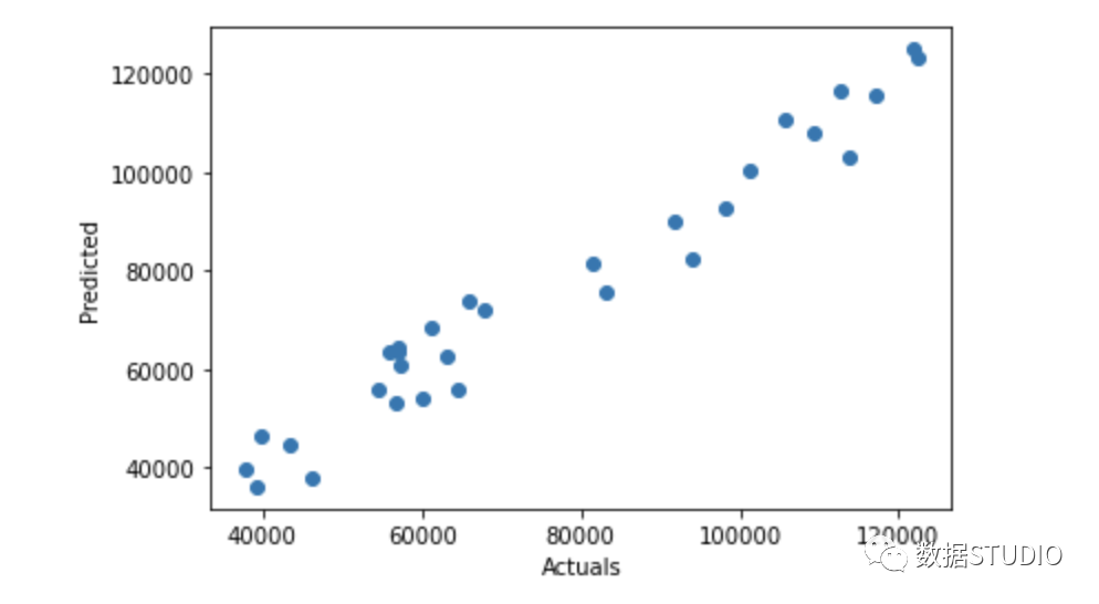
????plt.scatter(x=res['Actuals'],?y=res['Predicted'])
????plt.ylabel('Predicted')
????plt.xlabel('Actuals')
????
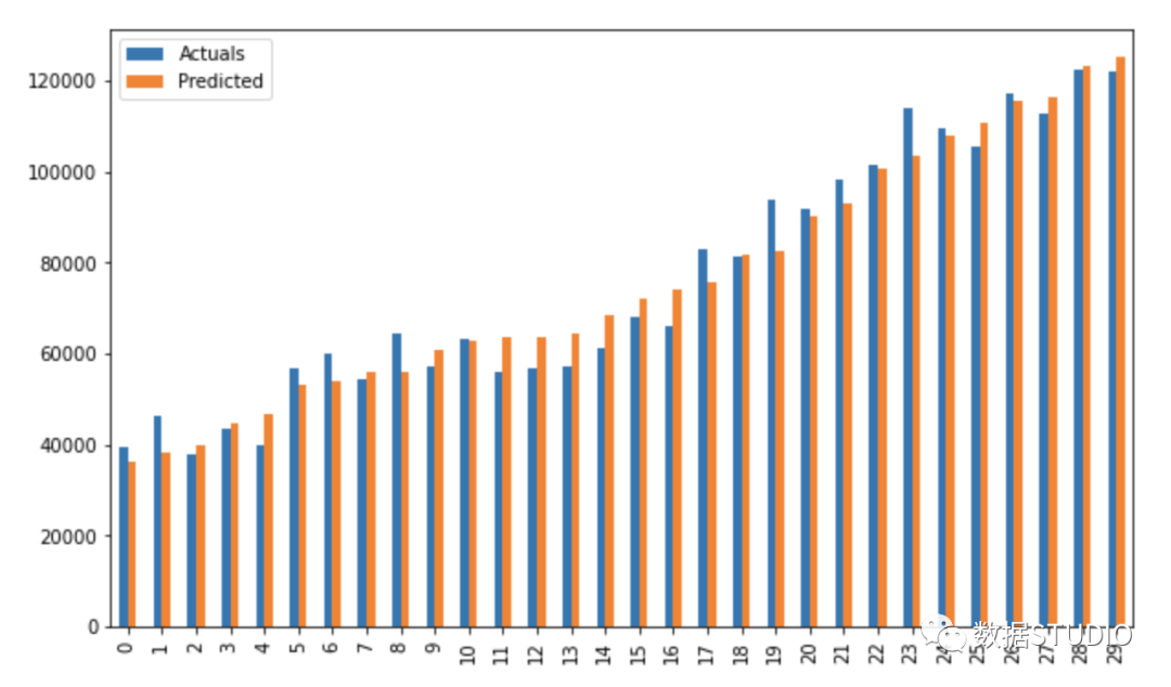
????res.plot(kind='bar',figsize=(10,6))

#?Driver?code
smf_ols(df[['Salary',?'YearsExperience']])?#?0.957?accuracy
#?smf_ols(df[['Norm_Salary',?'Norm_YearsExp']])?#?0.957?accuracy

使用 statsmodels.api 進(jìn)行回歸

不再需要單獨(dú)枚舉預(yù)測變量。

statsmodels.regression.linear_model.OLS(endog, exog)

• endog 是因變量
• exog是自變量。默認(rèn)情況下不包含截距項(xiàng)，應(yīng)由用戶使用 add_constant添加。

#?創(chuàng)建一個輔助函數(shù)
def?OLS_model(df):
????#?定義自變量和因變量
????x?=?df.iloc[:,?1:2]
????y?=?df.iloc[:,?0:1]?
????#?添加一個常數(shù)項(xiàng)
????x?=?sm.add_constant(x)
#?????print(x)
????model?=?sm.OLS(y,?x)
????#?訓(xùn)練模型
????results?=?model.fit()
????#?print('n'+"Confidence?interval:"+'n',?results.conf_int(alpha=0.05,?cols=None))?
????#?返回?cái)M合參數(shù)的置信區(qū)間。默認(rèn)alpha=0.05返回一個95%的置信區(qū)間。
????print('n'"Model?parameters:"+'n',results.params)
????#?打印model?summary
????print(results.summary())
????
#?Driver?code
OLS_model(df[['Salary',?'YearsExperience']])?#?0.957?accuracy
OLS_model(df[['Norm_Salary',?'Norm_YearsExp']])?#?0.957?accuracy

Model parameters:
 const              25792.200199
YearsExperience     9449.962321
dtype: float64

Model parameters:
 const            0.058395
Norm_YearsExp    0.703277
dtype: float64

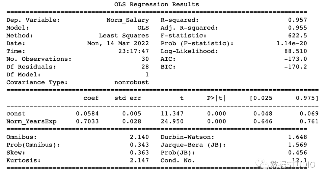
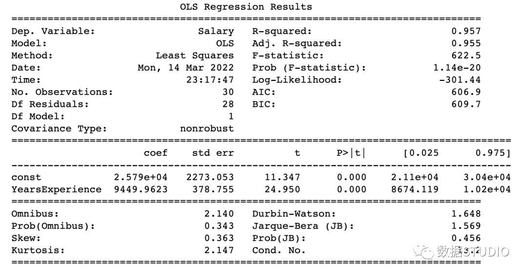
該模型達(dá)到了 95.7% 的準(zhǔn)確率，這是相當(dāng)不錯的。

如何讀懂 model summary

理解回歸模型model summary表中的某些術(shù)語總是很重要的，這樣我們才能了解模型的性能和輸入變量的相關(guān)性。

應(yīng)考慮的一些重要參數(shù)是 Adj. R-squared。R-squared，F(xiàn)-statistic，Prob（F-statistic），Intercept和輸入變量的coef，P>|t|。

• R-Squared是決定系數(shù)。一種統(tǒng)計(jì)方法，它表示有很大百分比的數(shù)據(jù)點(diǎn)落在最佳擬合線上。為使模型擬合良好，r2值接近1是預(yù)期的。
• Adj. R-squared 如果我們不斷添加對模型預(yù)測沒有貢獻(xiàn)的新特征，R-squared 會懲罰 R-squared 值。如果Adj. R-squared
• F-statistic 或者 F-test 幫助我們接受或拒絕零假設(shè)。它將僅截取模型與我們的具有特征的模型進(jìn)行比較。零假設(shè)是"所有回歸系數(shù)都等于 0，這意味著兩個模型都相等"。替代假設(shè)是“攔截唯一比我們的模型差的模型，這意味著我們添加的系數(shù)提高了模型性能。如果 prob(F-statistic) < 0.05 并且 F-statistic 是一個高值，我們拒絕零假設(shè)。它表示輸入變量和輸出變量之間存在良好的關(guān)系。
• coef 系數(shù)表示相應(yīng)輸入特征的估計(jì)系數(shù)
• T-test單獨(dú)討論輸出與每個輸入變量之間的關(guān)系。零假設(shè)是“輸入特征的系數(shù)為 0”。替代假設(shè)是“輸入特征的系數(shù)不為 0”。如果 pvalue < 0.05，我們拒絕原假設(shè)，這表明輸入變量和輸出變量之間存在良好的關(guān)系。我們可以消除 pvalue > 0.05 的變量。

到這里，我們應(yīng)該知道如何從model summary表中得出重要的推論了，那么現(xiàn)在看看模型參數(shù)并評估我們的模型。

在本例子中

1. R-Squared(0.957) 接近 Adj. R-squared ?(0.955) 是輸入特征對預(yù)測模型有貢獻(xiàn)的好兆頭。
2. F-statistic 是一個很大的數(shù)字，P(F-statistic) 幾乎為 0，這意味著我們的模型比唯一的截距模型要好。
3. 輸入變量t-test的pvalue小于0.05，所以輸入變量和輸出變量有很好的關(guān)系。

因此，我們得出結(jié)論說該模型效果良好！

到這里，本文就結(jié)束啦。今天和作者一起學(xué)習(xí)了簡單線性回歸 (SLR) 的基礎(chǔ)知識，使用不同的 Python 庫構(gòu)建線性模型，并從 OLS statsmodels 的model summary表中得出重要推論。