
顏色、形狀和紋理:使用 OpenCV 進行特征提取
圖像處理所做的只是從圖像中提取有用的信息,從而減少數(shù)據(jù)量,但保留描述圖像特征的像素。
1. 顏色
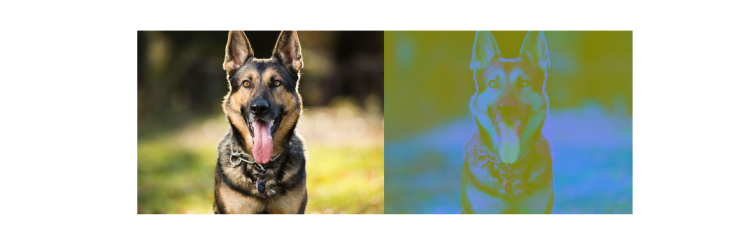
色調(diào):描述主波長,是指定顏色的通道 飽和度:描述色調(diào)/顏色的純度/色調(diào) 值:描述顏色的強度
import?cv2
from?google.colab.patches?import?cv2_imshow

image?=?cv2.imread(image_file)
hsv_image?=?cv2.cvtColor(image,?cv2.COLOR_BGR2HSV)
cv2_imshow(hsv_image)
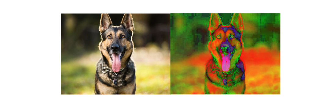
L:描述顏色的亮度,與強度互換使用 A : 顏色成分范圍,從綠色到品紅色 B:從藍色到黃色的顏色分量
import?cv2
from?google.colab.patches?import?cv2_imshow

image?=?cv2.imread(image_file)
lab_image?=?cv2.cvtColor(image,?cv2.COLOR_BGR2LAB)
cv2_imshow(lab_image)
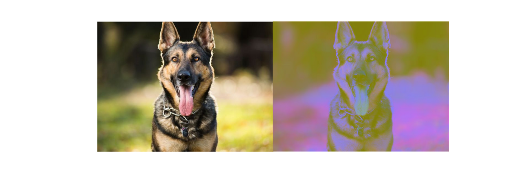
Y : 伽馬校正后從 RGB 顏色空間獲得的亮度 Cr:描述紅色 (R) 分量與亮度的距離 Cb:描述藍色 (B) 分量與亮度的距離
import?cv2
from?google.colab.patches?import?cv2_imshow

image?=?cv2.imread(image_file)
ycrcb_image?=?cv2.cvtColor(image,?cv2.COLOR_BGR2YCrCb)
cv2_imshow(ycrcb_image)
import?cv2
from?google.colab.patches?import?cv2_imshow
import?numpy?as?np
import?plotly.figure_factory?as?ff

#?Check?the?distribution?of?red?values?
red_values?=?[]
for?i?in?range(len(images)):
??red_value?=?np.mean(images[i][:,?:,?0])
??red_values.append(red_value)

#?Check?the?distribution?of?green?values?
green_values?=?[]
for?i?in?range(len(images)):
??green_value?=?np.mean(images[i][:,?:,?1])
??green_values.append(green_value)

#?Check?the?distribution?of?blue?values?
blue_values?=?[]
for?i?in?range(len(images)):
??blue_value?=?np.mean(images[i][:,?:,?2])
??blue_values.append(blue_value)
??
#?Plotting?the?histogram
fig?=?ff.create_distplot([red_values,?green_values,?blue_values],?group_labels=["R",?"G",?"B"],?colors=['red',?'green',?'blue'])
fig.update_layout(showlegend=True,?template="simple_white")
fig.update_layout(title_text='Distribution?of?channel?values?across?images?in?RGB')
fig.data[0].marker.line.color?=?'rgb(0,?0,?0)'
fig.data[0].marker.line.width?=?0.5
fig.data[1].marker.line.color?=?'rgb(0,?0,?0)'
fig.data[1].marker.line.width?=?0.5
fig.data[2].marker.line.color?=?'rgb(0,?0,?0)'
fig.data[2].marker.line.width?=?0.5
fig
import?cv2
from?google.colab.patches?import?cv2_imshow
#?Reading?the?original?image
image_spot?=?cv2.imread(image_file)
cv2_imshow(image_spot)
#?Converting?it?to?HSV?color?space
hsv_image_spot?=?cv2.cvtColor(image_spot,?cv2.COLOR_BGR2HSV)
cv2_imshow(hsv_image_spot)
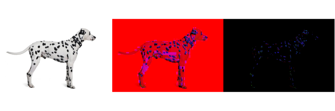
#?Setting?the?black?pixel?mask?and?perform?bitwise_and?to?get?only?the?black?pixels
mask?=?cv2.inRange(hsv_image_spot,?(0,?0,?0),?(180,?255,?40))
masked?=?cv2.bitwise_and(hsv_image_spot,?hsv_image_spot,?mask=mask)
cv2_imshow(masked)
import?cv2
from?google.colab.patches?import?cv2_imshow

image_spot_reshaped?=?image_spot.reshape((image_spot.shape[0]?*?image_spot.shape[1],?3))

#?convert?to?np.float32
Z?=?np.float32(image_spot_reshaped)
#?define?criteria,?number?of?clusters(K)?and?apply?kmeans()
criteria?=?(cv2.TERM_CRITERIA_EPS?+?cv2.TERM_CRITERIA_MAX_ITER,?10,?1.0)
K?=?2
ret,?label,?center?=?cv2.kmeans(Z,?K,?None,?criteria,?10,?cv2.KMEANS_RANDOM_CENTERS)
#?Now?convert?back?into?uint8,?and?make?original?image
center?=?np.uint8(center)
res?=?center[label.flatten()]
res2?=?res.reshape((image_spot.shape))

cv2_imshow(res2)
2. 形狀
矩 輪廓面積 輪廓周長 輪廓近似 凸包 凸性檢測 矩形邊界 最小外接圓 擬合橢圓 擬合直線
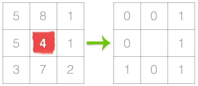
3. 紋理
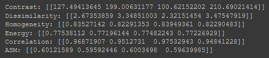
對比度:測量灰度共生矩陣的局部變化。 相關(guān)性:測量指定像素對的聯(lián)合概率出現(xiàn)。 平方:提供 GLCM 中元素的平方和。也稱為均勻性或角二階矩。 同質(zhì)性:測量 GLCM 中元素分布與 GLCM 對角線的接近程度。
import?cv2
from?google.colab.patches?import?cv2_imshow

image_spot?=?cv2.imread(image_file)
gray?=?cv2.cvtColor(image_spot,?cv2.COLOR_BGR2GRAY)

#?Find?the?GLCM
import?skimage.feature?as?feature

#?Param:
#?source?image
#?List?of?pixel?pair?distance?offsets?-?here?1?in?each?direction
#?List?of?pixel?pair?angles?in?radians
graycom?=?feature.greycomatrix(gray,?[1],?[0,?np.pi/4,?np.pi/2,?3*np.pi/4],?levels=256)

#?Find?the?GLCM?properties
contrast?=?feature.greycoprops(graycom,?'contrast')
dissimilarity?=?feature.greycoprops(graycom,?'dissimilarity')
homogeneity?=?feature.greycoprops(graycom,?'homogeneity')
energy?=?feature.greycoprops(graycom,?'energy')
correlation?=?feature.greycoprops(graycom,?'correlation')
ASM?=?feature.greycoprops(graycom,?'ASM')

print("Contrast:?{}".format(contrast))
print("Dissimilarity:?{}".format(dissimilarity))
print("Homogeneity:?{}".format(homogeneity))
print("Energy:?{}".format(energy))
print("Correlation:?{}".format(correlation))
print("ASM:?{}".format(ASM))
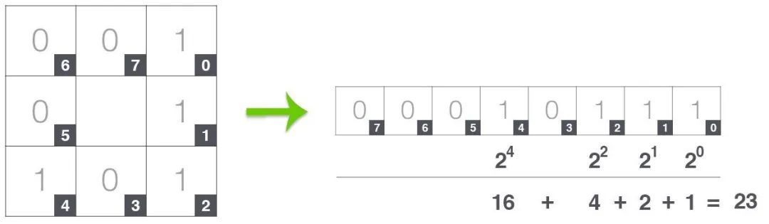
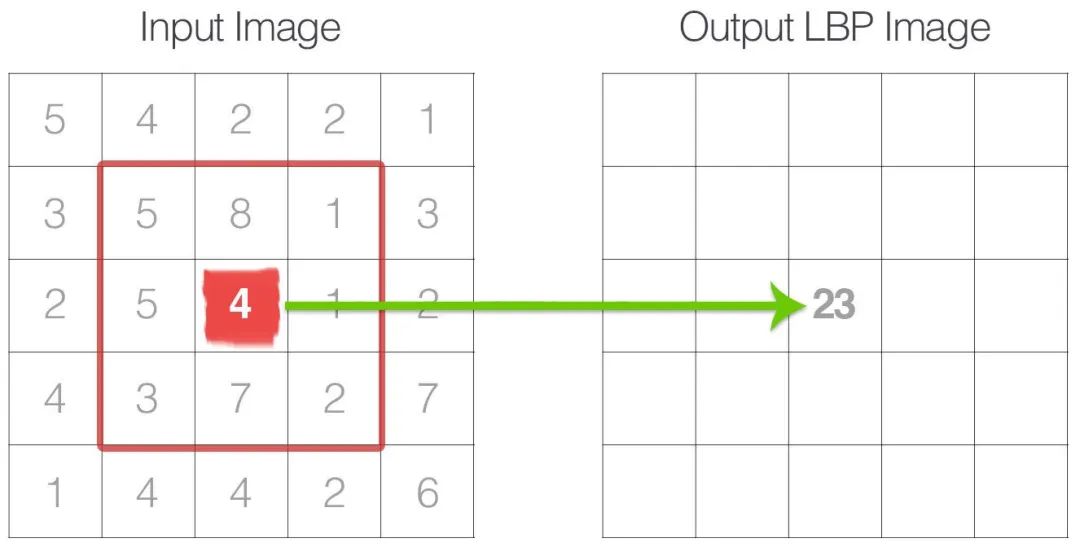
https://www.pyimagesearch.com/2015/12/07/local-binary-patterns-with-python-opencv/ https://towardsdatascience.com/face-recognition-how-lbph-works-90ec258c3d6b
import?cv2
from?google.colab.patches?import?cv2_imshow
class?LocalBinaryPatterns:
??def?__init__(self,?numPoints,?radius):
????self.numPoints?=?numPoints
????self.radius?=?radius
??def?describe(self,?image,?eps?=?1e-7):
????lbp?=?feature.local_binary_pattern(image,?self.numPoints,?self.radius,?method="uniform")
????(hist,?_)?=?np.histogram(lbp.ravel(),?bins=np.arange(0,?self.numPoints+3),?range=(0,?self.numPoints?+?2))
????#?Normalize?the?histogram
????hist?=?hist.astype('float')
????hist?/=?(hist.sum()?+?eps)
????return?hist,?lbp
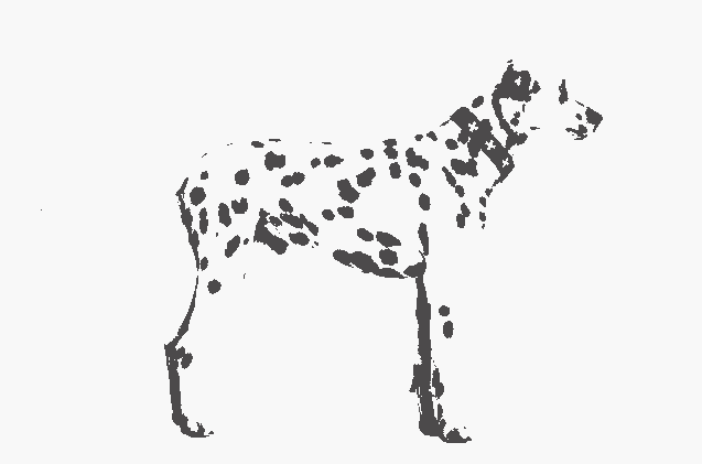
image?=?cv2.imread(image_file)
gray?=?cv2.cvtColor(image,?cv2.COLOR_BGR2GRAY)
desc?=?LocalBinaryPatterns(24,?8)
hist,?lbp?=?desc.describe(gray)
print("Histogram?of?Local?Binary?Pattern?value:?{}".format(hist))
contrast?=?contrast.flatten()
dissimilarity?=?dissimilarity.flatten()
homogeneity?=?homogeneity.flatten()
energy?=?energy.flatten()
correlation?=?correlation.flatten()
ASM?=?ASM.flatten()
hist?=?hist.flatten()
features?=?np.concatenate((contrast,?dissimilarity,?homogeneity,?energy,?correlation,?ASM,?hist),?axis=0)?
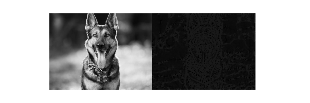
cv2_imshow(gray)
cv2_imshow(lbp)
結(jié)論
參考
https://www.analyticsvidhya.com/blog/2019/08/3-techniques-extract-features-from-image-data-machine-learning-python/ https://www.mygreatlearning.com/blog/feature-extraction-in-image-processing/ https://thevatsalsaglani.medium.com/feature-extraction-from-medical-images-and-an-introduction-to-xtract-features-9a225243e94b http://www.scholarpedia.org/article/Local_Binary_Patterns https://medium.com/mlearning-ai/mlearning-ai-submission-suggestions-b51e2b130bfb
評論
圖片
表情