
詳解蒙特卡洛方法:這些數(shù)學你搞懂了嗎?

極市導讀
?加州大學洛杉磯分校計算機科學專業(yè)的 Ray Zhang 最近開始在自己的博客上連載介紹強化學習的文章,這些介紹文章主要基于 Richard S. Sutton 和 Andrew G. Barto 合著的《Reinforcement Learning: an Introduction》,并添加了一些示例說明。該系列文章現(xiàn)已介紹了賭博機問題、馬爾可夫決策過程和蒙特卡洛方法。本文是對其中蒙特卡洛方法文章的編譯。>>加入極市CV技術交流群,走在計算機視覺的最前沿
目錄
first-visit 蒙特卡洛
探索開始
在策略:?-貪婪策略
?-貪婪收斂?
離策略:重要度采樣
離策略標記法
普通重要度采樣
加權重要度采樣
增量實現(xiàn)
其它:可感知折扣的重要度采樣
其它:預獎勵重要度采樣
示例:Blackjack
示例:Cliff Walking
 和
和 的算法。我們使用了策略迭代和價值迭代來求解最優(yōu)策略。
引言

 ?與可能的
?與可能的 ?關聯(lián)起來,以推導某種類型的:
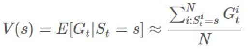

pi = init_pi()
returns = defaultdict(list)
for i in range(NUM_ITER):
 ? ?episode = generate_episode(pi) # (1)
 ? ?G = np.zeros(|S|)
 ? ?prev_reward = 0
 ? ?for (state, reward) in reversed(episode):
 ? ? ? ?reward += GAMMA * prev_reward
 ? ? ? ?# backing up replaces s eventually,
 ? ? ? ?# so we get first-visit reward.
 ? ? ? ?G[s] = reward
 ? ? ? ?prev_reward = reward
 ? ?for state in STATES:
 ? ? ? ?returns[state].append(state)
V = { state : np.mean(ret) for state, ret in returns.items() }
蒙特卡洛動作值
 而非
而非 。將 G[s] 簡單地改成 G[s,a] 似乎很恰當,事實也確實如此。一個顯然的問題是:現(xiàn)在我們從 S 空間變成了 S×A 空間,這會大很多,而且我們?nèi)匀恍枰獙ζ溥M行采樣以找到每個狀態(tài)-動作元組的期望回報。
蒙特卡洛控制
 ,然后尋找一個新的 π′ 再繼續(xù)。大致過程就像這樣:
 的方式類似于上面我們尋找 v 的方式。我們可以通過貝爾曼最優(yōu)性方程(Bellman optimality equation)的定義改善我們的 π,簡單來說就是:
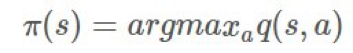
# Before (Start at some arbitrary s_0, a_0)
episode = generate_episode(pi)
# After (Start at some specific s, a)
episode = generate_episode(pi, s, a) # loop through s, a at every iteration.
 ?動作。
?動作。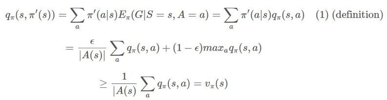
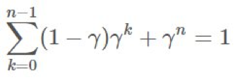
 ?上執(zhí)行單調(diào)的提升。如果我們支持所有時間步驟,那么會得到:
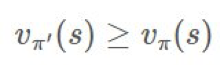
 ,則由于該環(huán)境的設置,方程在隨機性下是最優(yōu)的。
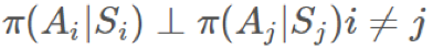
π 是我們的目標策略(target policy)。我們試圖優(yōu)化這個策略的期望回報。
b 是我們的行為策略(behavioral policy)。我們使用 b 來生成 π 之后會用到的數(shù)據(jù)。
 這是覆蓋率(coverage)的概念。
 ,則
,則 是怎樣的?」換句話說,你該怎樣使用你從 b 的采樣得到的信息來確定來自 π 的期望結果?
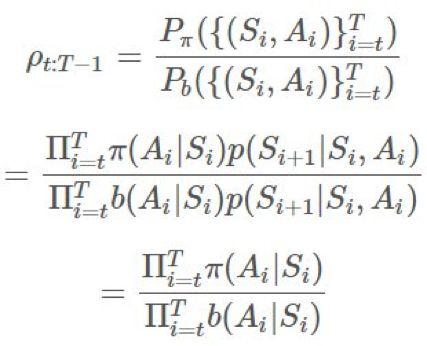
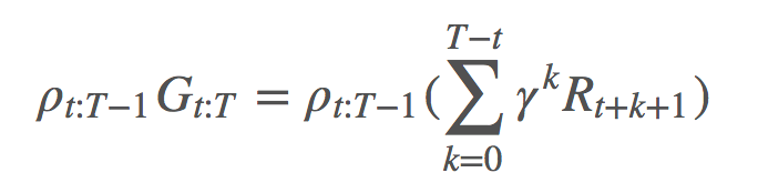
 ,這個確切軌跡在給定策略 π 時的概率為:
 的方法,以給我們提供一個
 ?的優(yōu)良估計。最基本的方法是使用被稱為普通重要度采樣(ordinary importance sampling)的技術。假設我們有采樣得到的 N 個 episode:
 ,然后我們可以通過 first-visit 方法使用實驗的均值來估計價值函數(shù):
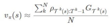
 是 1000。這是個很大的比值,但絕對有可能發(fā)生。這是否意味著獎勵必然會多 1000 倍?如果我們只有 1 個 episode,我們的估計就會是那樣。在長期運行時,因為我們有乘法關系,所以這個比值可能要么會爆炸,要么就會消失。這對估計的目的而言是有一點問題的。
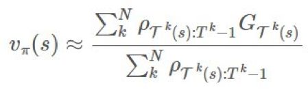
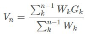
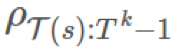
 是我們的權重。
 ?構建
?構建 ,這是非常可行的。用
 ?表示
?表示 ,則我們可以保持這個運行總和的更新,即:
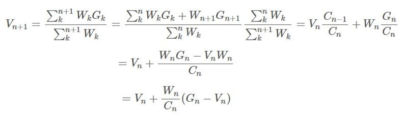 ?的更新規(guī)則相當明顯:
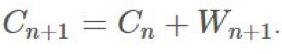
 ?是我們的價值函數(shù),但在我們的動作值
 ?上也可以應用一個非常類似的類比。
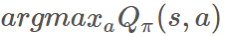 更新我們的 π。
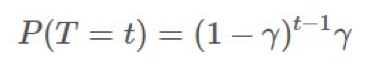
 的隨機數(shù)上的期望:
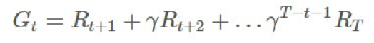
 。
。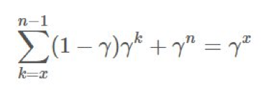
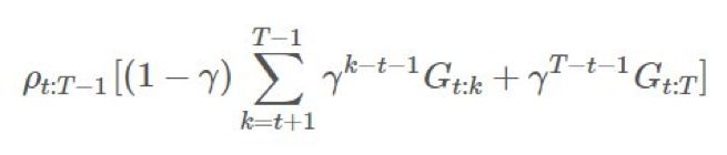
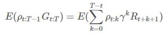
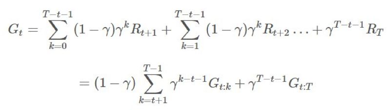 ?項上的等效系數(shù)為 1、γ、γ2。這意味著我們現(xiàn)在可將
 ?分解成不同的部分并在重要度采樣比上應用折扣。
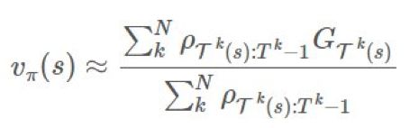
 乘上了整個軌跡的重要度比,這在「γ 是終止概率」的建模假設下是「不正確的」。直觀來看,我們希望?有
 ,這是很簡單的:
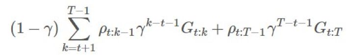
 :
:
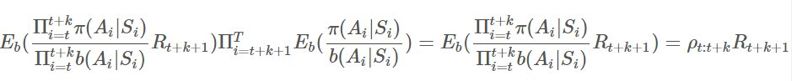
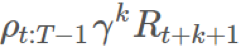 。擴展 ρ,我們可以看到:
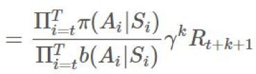
 的期望:
的期望: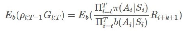
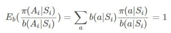
 ,那么任何
,那么任何 和
和 獨立于
獨立于 (對 b 的情況也一樣)。我們可以將它們?nèi)〕觯缓蟮玫剑?/span>
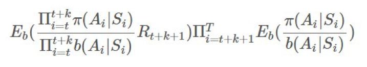
用 Python 實現(xiàn)的在策略模型
"""
General purpose Monte Carlo model for training on-policy methods.
"""
from copy import deepcopy
import numpy as np

class FiniteMCModel:
 ? ?def __init__(self, state_space, action_space, gamma=1.0, epsilon=0.1):
 ? ? ? ?"""MCModel takes in state_space and action_space (finite)
 ? ? ? ?Arguments
 ? ? ? ?---------

 ? ? ? ?state_space: int OR list[observation], where observation is any hashable type from env's obs.
 ? ? ? ?action_space: int OR list[action], where action is any hashable type from env's actions.
 ? ? ? ?gamma: float, discounting factor.
 ? ? ? ?epsilon: float, epsilon-greedy parameter.

 ? ? ? ?If the parameter is an int, then we generate a list, and otherwise we generate a dictionary.
 ? ? ? ?>>> m = FiniteMCModel(2,3,epsilon=0)
 ? ? ? ?>>> m.Q
 ? ? ? ?[[0, 0, 0], [0, 0, 0]]
 ? ? ? ?>>> m.Q[0][1] = 1
 ? ? ? ?>>> m.Q
 ? ? ? ?[[0, 1, 0], [0, 0, 0]]
 ? ? ? ?>>> m.pi(1, 0)
 ? ? ? ?1
 ? ? ? ?>>> m.pi(1, 1)
 ? ? ? ?0
 ? ? ? ?>>> d = m.generate_returns([(0,0,0), (0,1,1), (1,0,1)])
 ? ? ? ?>>> assert(d == {(1, 0): 1, (0, 1): 2, (0, 0): 2})
 ? ? ? ?>>> m.choose_action(m.pi, 1)
 ? ? ? ?0
 ? ? ? ?"""
 ? ? ? ?self.gamma = gamma
 ? ? ? ?self.epsilon = epsilon
 ? ? ? ?self.Q = None
 ? ? ? ?if isinstance(action_space, int):
 ? ? ? ? ? ?self.action_space = np.arange(action_space)
 ? ? ? ? ? ?actions = [0]*action_space
 ? ? ? ? ? ?# Action representation
 ? ? ? ? ? ?self._act_rep = "list"
 ? ? ? ?else:
 ? ? ? ? ? ?self.action_space = action_space
 ? ? ? ? ? ?actions = {k:0 for k in action_space}
 ? ? ? ? ? ?self._act_rep = "dict"
 ? ? ? ?if isinstance(state_space, int):
 ? ? ? ? ? ?self.state_space = np.arange(state_space)
 ? ? ? ? ? ?self.Q = [deepcopy(actions) for _ in range(state_space)]
 ? ? ? ?else:
 ? ? ? ? ? ?self.state_space = state_space
 ? ? ? ? ? ?self.Q = {k:deepcopy(actions) for k in state_space}

 ? ? ? ?# Frequency of state/action.
 ? ? ? ?self.Ql = deepcopy(self.Q)


 ? ?def pi(self, action, state):
 ? ? ? ?"""pi(a,s,A,V) := pi(a|s)
 ? ? ? ?We take the argmax_a of Q(s,a).
 ? ? ? ?q[s] = [q(s,0), q(s,1), ...]
 ? ? ? ?"""
 ? ? ? ?if self._act_rep == "list":
 ? ? ? ? ? ?if action == np.argmax(self.Q[state]):
 ? ? ? ? ? ? ? ?return 1
 ? ? ? ? ? ?return 0
 ? ? ? ?elif self._act_rep == "dict":
 ? ? ? ? ? ?if action == max(self.Q[state], key=self.Q[state].get):
 ? ? ? ? ? ? ? ?return 1
 ? ? ? ? ? ?return 0


 ? ?def b(self, action, state):
 ? ? ? ?"""b(a,s,A) := b(a|s)
 ? ? ? ?Sometimes you can only use a subset of the action space
 ? ? ? ?given the state.

 ? ? ? ?Randomly selects an action from a uniform distribution.
 ? ? ? ?"""
 ? ? ? ?return self.epsilon/len(self.action_space) + (1-self.epsilon) * self.pi(action, state)


 ? ?def generate_returns(self, ep):
 ? ? ? ?"""Backup on returns per time period in an epoch
 ? ? ? ?Arguments
 ? ? ? ?---------

 ? ? ? ?ep: [(observation, action, reward)], an episode trajectory in chronological order.
 ? ? ? ?"""
 ? ? ? ?G = {} # return on state
 ? ? ? ?C = 0 # cumulative reward
 ? ? ? ?for tpl in reversed(ep):
 ? ? ? ? ? ?observation, action, reward = tpl
 ? ? ? ? ? ?G[(observation, action)] = C = reward + self.gamma*C
 ? ? ? ?return G


 ? ?def choose_action(self, policy, state):
 ? ? ? ?"""Uses specified policy to select an action randomly given the state.
 ? ? ? ?Arguments
 ? ? ? ?---------

 ? ? ? ?policy: function, can be self.pi, or self.b, or another custom policy.
 ? ? ? ?state: observation of the environment.
 ? ? ? ?"""
 ? ? ? ?probs = [policy(a, state) for a in self.action_space]
 ? ? ? ?return np.random.choice(self.action_space, p=probs)


 ? ?def update_Q(self, ep):
 ? ? ? ?"""Performs a action-value update.
 ? ? ? ?Arguments
 ? ? ? ?---------

 ? ? ? ?ep: [(observation, action, reward)], an episode trajectory in chronological order.
 ? ? ? ?"""
 ? ? ? ?# Generate returns, return ratio
 ? ? ? ?G = self.generate_returns(ep)
 ? ? ? ?for s in G:
 ? ? ? ? ? ?state, action = s
 ? ? ? ? ? ?q = self.Q[state][action]
 ? ? ? ? ? ?self.Ql[state][action] += 1
 ? ? ? ? ? ?N = self.Ql[state][action]
 ? ? ? ? ? ?self.Q[state][action] = q * N/(N+1) + G[s]/(N+1)

 ? ?def score(self, env, policy, n_samples=1000):
 ? ? ? ?"""Evaluates a specific policy with regards to the env.
 ? ? ? ?Arguments
 ? ? ? ?---------

 ? ? ? ?env: an openai gym env, or anything that follows the api.
 ? ? ? ?policy: a function, could be self.pi, self.b, etc.
 ? ? ? ?"""
 ? ? ? ?rewards = []
 ? ? ? ?for _ in range(n_samples):
 ? ? ? ? ? ?observation = env.reset()
 ? ? ? ? ? ?cum_rewards = 0
 ? ? ? ? ? ?while True:
 ? ? ? ? ? ? ? ?action = self.choose_action(policy, observation)
 ? ? ? ? ? ? ? ?observation, reward, done, _ = env.step(action)
 ? ? ? ? ? ? ? ?cum_rewards += reward
 ? ? ? ? ? ? ? ?if done:
 ? ? ? ? ? ? ? ? ? ?rewards.append(cum_rewards)
 ? ? ? ? ? ? ? ? ? ?break
 ? ? ? ?return np.mean(rewards)

if __name__ == "__main__":
 ? ?import doctest
 ? ?doctest.testmod()
import gym
env = gym.make("Blackjack-v0")
# The typical imports
import gym
import numpy as np
import matplotlib.pyplot as plt
from mc import FiniteMCModel as MC
eps = 1000000
S = [(x, y, z) for x in range(4,22) for y in range(1,11) for z in [True,False]]
A = 2
m = MC(S, A, epsilon=1)
for i in range(1, eps+1):
? ?ep = []
? ?observation = env.reset()
? ?while True:
? ? ? ?# Choosing behavior policy
? ? ? ?action = m.choose_action(m.b, observation)
? ? ? ?# Run simulation
? ? ? ?next_observation, reward, done, _ = env.step(action)
? ? ? ?ep.append((observation, action, reward))
? ? ? ?observation = next_observation
? ? ? ?if done:
? ? ? ? ? ?break
? ?m.update_Q(ep)
? ?# Decaying epsilon, reach optimal policy
? ?m.epsilon = max((eps-i)/eps, 0.1)
print("Final expected returns : {}".format(m.score(env, m.pi, n_samples=10000)))
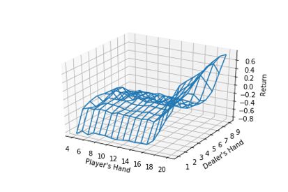
# plot a 3D wireframe like in the example mplot3d/wire3d_demo
X = np.arange(4, 21)
Y = np.arange(1, 10)
Z = np.array([np.array([m.Q[(x, y, False)][0] for x in X]) for y in Y])
X, Y = np.meshgrid(X, Y)
from mpl_toolkits.mplot3d.axes3d import Axes3D
fig = plt.figure()
ax = fig.add_subplot(111, projection='3d')
ax.plot_wireframe(X, Y, Z, rstride=1, cstride=1)
ax.set_xlabel("Player's Hand")
ax.set_ylabel("Dealer's Hand")
ax.set_zlabel("Return")
plt.savefig("blackjackpolicy.png")
plt.show()
Iterations: 100/1k/10k/100k/1million.
Tested on 10k samples for expected returns.

On-policy : greedy
-0.1636
-0.1063
-0.0648
-0.0458
-0.0312

On-policy : eps-greedy with eps=0.3
-0.2152
-0.1774
-0.1248
-0.1268
-0.1148

Off-policy weighted importance sampling:
-0.2393
-0.1347
-0.1176
-0.0813
-0.072
# Before: Blackjack-v0
env = gym.make("CliffWalking-v0")
# Before: [(x, y, z) for x in range(4,22) for y in range(1,11) for z in [True,False]]
S = 4*12
# Before: 2
A = 4
總結
推薦閱讀

評論
圖片
表情