
如何從NumPy直接創(chuàng)建RNN?
(點(diǎn)擊上方快速關(guān)注并設(shè)置為星標(biāo),一起學(xué)Python)
木易 發(fā)自 凹非寺?
量子位 報道 | 公眾號 QbitAI
使用成熟的Tensorflow、PyTorch框架去實(shí)現(xiàn)遞歸神經(jīng)網(wǎng)絡(luò)(RNN),已經(jīng)極大降低了技術(shù)的使用門檻。
但是,對于初學(xué)者,這還是遠(yuǎn)遠(yuǎn)不夠的。知其然,更需知其所以然。

要避免低級錯誤,打好理論基礎(chǔ),然后使用RNN去解決更多實(shí)際的問題的話。
那么,有一個有趣的問題可以思考一下:
不使用Tensorflow等框架,只有Numpy的話,你該如何構(gòu)建RNN?
沒有頭緒也不用擔(dān)心。這里便有一項教程:使用Numpy從頭構(gòu)建用于NLP領(lǐng)域的RNN。
可以帶你行進(jìn)一遍RNN的構(gòu)建流程。
初始化參數(shù)
與傳統(tǒng)的神經(jīng)網(wǎng)絡(luò)不同,RNN具有3個權(quán)重參數(shù),即:
輸入權(quán)重(input weights),內(nèi)部狀態(tài)權(quán)重(internal state weights)和輸出權(quán)重(output weights)
首先用隨機(jī)數(shù)值初始化上述三個參數(shù)。
之后,將詞嵌入維度(word_embedding dimension)和輸出維度(output dimension)分別初始化為100和80。
輸出維度是詞匯表中存在的唯一詞向量的總數(shù)。
hidden_dim?=?100???????
output_dim?=?80?#?this?is?the?total?unique?words?in?the?vocabulary
input_weights?=?np.random.uniform(0,?1,?(hidden_dim,hidden_dim))
internal_state_weights?=?np.random.uniform(0,1,?(hidden_dim,?hidden_dim))
output_weights?=?np.random.uniform(0,1,?(output_dim,hidden_dim))
變量prev_memory指的是internal_state(這些是先前序列的內(nèi)存)。
其他參數(shù)也給予了初始化數(shù)值。
input_weight梯度,internal_state_weight梯度和output_weight梯度分別命名為dU,dW和dV。
變量bptt_truncate表示網(wǎng)絡(luò)在反向傳播時必須回溯的時間戳數(shù),這樣做是為了克服梯度消失的問題。
prev_memory?=??np.zeros((hidden_dim,1))
learning_rate?=?0.0001????
nepoch?=?25???????????????
T?=?4???#?length?of?sequence
bptt_truncate?=?2?
dU?=?np.zeros(input_weights.shape)
dV?=?np.zeros(output_weights.shape)
dW?=?np.zeros(internal_state_weights.shape)
前向傳播
輸出和輸入向量
例如有一句話為:I like to play.,則假設(shè)在詞匯表中:
I被映射到索引2,like對應(yīng)索引45,to對應(yīng)索引10、**對應(yīng)索引64而標(biāo)點(diǎn)符號.** 對應(yīng)索引1。
為了展示從輸入到輸出的情況,我們先隨機(jī)初始化每個單詞的詞嵌入。
input_string?=?[2,45,10,65]
embeddings?=?[]?#?this?is?the?sentence?embedding?list?that?contains?the?embeddings?for?each?word
for?i?in?range(0,T):
????x?=?np.random.randn(hidden_dim,1)
????embeddings.append(x)
輸入已經(jīng)完成,接下來需要考慮輸出。
在本項目中,RNN單元接受輸入后,輸出的是下一個最可能出現(xiàn)的單詞。
用于訓(xùn)練RNN,在給定第t+1個詞作為輸出的時候?qū)⒌趖個詞作為輸入,例如:在RNN單元輸出字為“l(fā)ike”的時候給定的輸入字為“I”.
現(xiàn)在輸入是嵌入向量的形式,而計算損失函數(shù)(Loss)所需的輸出格式是獨(dú)熱編碼(One-Hot)矢量。
這是對輸入字符串中除第一個單詞以外的每個單詞進(jìn)行的操作,因為該神經(jīng)網(wǎng)絡(luò)學(xué)習(xí)只學(xué)習(xí)的是一個示例句子,而初始輸入是該句子的第一個單詞。
RNN的黑箱計算
現(xiàn)在有了權(quán)重參數(shù),也知道輸入和輸出,于是可以開始前向傳播的計算。
訓(xùn)練神經(jīng)網(wǎng)絡(luò)需要以下計算:
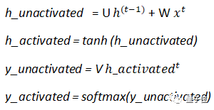
其中:
U代表輸入權(quán)重、W代表內(nèi)部狀態(tài)權(quán)重,V代表輸出權(quán)重。
輸入權(quán)重乘以input(x),內(nèi)部狀態(tài)權(quán)重乘以前一層的激活(prev_memory)。
層與層之間使用的激活函數(shù)用的是tanh。
def?tanh_activation(Z):
?????return?(np.exp(Z)-np.exp(-Z))/(np.exp(Z)-np.exp(-Z))?#?this?is?the?tanh?function?can?also?be?written?as?np.tanh(Z)
def?softmax_activation(Z):
????????e_x?=?np.exp(Z?-?np.max(Z))??#?this?is?the?code?for?softmax?function?
????????return?e_x?/?e_x.sum(axis=0)?
def?Rnn_forward(input_embedding,?input_weights,?internal_state_weights,?prev_memory,output_weights):
????forward_params?=?[]
????W_frd?=?np.dot(internal_state_weights,prev_memory)
????U_frd?=?np.dot(input_weights,input_embedding)
????sum_s?=?W_frd?+?U_frd
????ht_activated?=?tanh_activation(sum_s)
????yt_unactivated?=?np.asarray(np.dot(output_weights,??tanh_activation(sum_s)))
????yt_activated?=?softmax_activation(yt_unactivated)
????forward_params.append([W_frd,U_frd,sum_s,yt_unactivated])
????return?ht_activated,yt_activated,forward_params
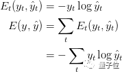
計算損失函數(shù)
之后損失函數(shù)使用的是交叉熵?fù)p失函數(shù),由下式給出:
def?calculate_loss(output_mapper,predicted_output):
????total_loss?=?0
????layer_loss?=?[]
????for?y,y_?in?zip(output_mapper.values(),predicted_output):?#?this?for?loop?calculation?is?for?the?first?equation,?where?loss?for?each?time-stamp?is?calculated
????????loss?=?-sum(y[i]*np.log2(y_[i])?for?i?in?range(len(y)))
????????loss?=?loss/?float(len(y))
????????layer_loss.append(loss)?
????for?i?in?range(len(layer_loss)):?#this?the?total?loss?calculated?for?all?the?time-stamps?considered?together.?
????????total_loss??=?total_loss?+?layer_loss[i]
????return?total_loss/float(len(predicted_output))
最重要的是,我們需要在上面的代碼中看到第5行。
正如所知,ground_truth output(y)的形式是[0,0,….,1,…0]和predicted_output(y^hat)是[0.34,0.03,……,0.45]的形式,我們需要損失是單個值來從它推斷總損失。
為此,使用sum函數(shù)來獲得特定時間戳下y和y^hat向量中每個值的誤差之和。
total_loss是整個模型(包括所有時間戳)的損失。
反向傳播
反向傳播的鏈?zhǔn)椒▌t:
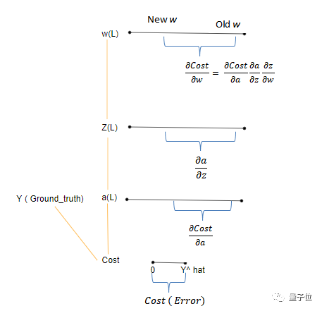
如上圖所示:
Cost代表誤差,它表示的是y^hat到y(tǒng)的差值。
由于Cost是的函數(shù)輸出,因此激活a所反映的變化由dCost/da表示。
實(shí)際上,這意味著從激活節(jié)點(diǎn)的角度來看這個變化(誤差)值。
類似地,a相對于z的變化表示為da/dz,z相對于w的變化表示為dw/dz。
最終,我們關(guān)心的是權(quán)重的變化(誤差)有多大。
而由于權(quán)重與Cost之間沒有直接關(guān)系,因此期間各個相對的變化值可以直接相乘(如上式所示)。
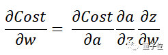
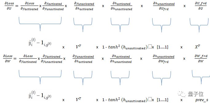
RNN的反向傳播
由于RNN中存在三個權(quán)重,因此我們需要三個梯度。input_weights(dLoss / dU),internal_state_weights(dLoss / dW)和output_weights(dLoss / dV)的梯度。
這三個梯度的鏈可以表示如下:
所述dLoss/dy_unactivated代碼如下:
def?delta_cross_entropy(predicted_output,original_t_output):
????li?=?[]
????grad?=?predicted_output
????for?i,l?in?enumerate(original_t_output):?#check?if?the?value?in?the?index?is?1?or?not,?if?yes?then?take?the?same?index?value?from?the?predicted_ouput?list?and?subtract?1?from?it.?
????????if?l?==?1:
????#grad?=?np.asarray(np.concatenate(?grad,?axis=0?))
????????????grad[i]?-=?1
????return?grad
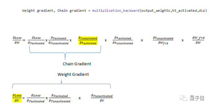
計算兩個梯度函數(shù),一個是multiplication_backward,另一個是additional_backward。
在multiplication_backward的情況下,返回2個參數(shù),一個是相對于權(quán)重的梯度(dLoss / dV),另一個是鏈梯度(chain gradient),該鏈梯度將成為計算另一個權(quán)重梯度的鏈的一部分。
在addition_backward的情況下,在計算導(dǎo)數(shù)時,加法函數(shù)(ht_unactivated)中各個組件的導(dǎo)數(shù)為1。例如:dh_unactivated / dU_frd=1(h_unactivated = U_frd + W_frd),且dU_frd / dU_frd的導(dǎo)數(shù)為1。
所以,計算梯度只需要這兩個函數(shù)。multiplication_backward函數(shù)用于包含向量點(diǎn)積的方程,addition_backward用于包含兩個向量相加的方程。
def?multiplication_backward(weights,x,dz):
????gradient_weight?=?np.array(np.dot(np.asmatrix(dz),np.transpose(np.asmatrix(x))))
????chain_gradient?=?np.dot(np.transpose(weights),dz)
????return?gradient_weight,chain_gradient

def?add_backward(x1,x2,dz):????#?this?function?is?for?calculating?the?derivative?of?ht_unactivated?function
????dx1?=?dz?*?np.ones_like(x1)
????dx2?=?dz?*?np.ones_like(x2)
????return?dx1,dx2

def?tanh_activation_backward(x,top_diff):
????output?=?np.tanh(x)
????return?(1.0?-?np.square(output))?*?top_diff
至此,已經(jīng)分析并理解了RNN的反向傳播,目前它是在單個時間戳上實(shí)現(xiàn)它的功能,之后可以將其用于計算所有時間戳上的梯度。
如下面的代碼所示,forward_params_t是一個列表,其中包含特定時間步長的網(wǎng)絡(luò)的前向參數(shù)。
變量ds是至關(guān)重要的部分,因為此行代碼考慮了先前時間戳的隱藏狀態(tài),這將有助于提取在反向傳播時所需的信息。
def?single_backprop(X,input_weights,internal_state_weights,output_weights,ht_activated,dLo,forward_params_t,diff_s,prev_s):#?inlide?all?the?param?values?for?all?the?data?thats?there
????W_frd?=?forward_params_t[0][0]?
????U_frd?=?forward_params_t[0][1]
????ht_unactivated?=?forward_params_t[0][2]
????yt_unactivated?=?forward_params_t[0][3]
????dV,dsv?=?multiplication_backward(output_weights,ht_activated,dLo)
????ds?=?np.add(dsv,diff_s)?#?used?for?truncation?of?memory?
????dadd?=?tanh_activation_backward(ht_unactivated,?ds)
????dmulw,dmulu?=?add_backward(U_frd,W_frd,dadd)
????dW,?dprev_s?=?multiplication_backward(internal_state_weights,?prev_s?,dmulw)
????dU,?dx?=?multiplication_backward(input_weights,?X,?dmulu)?#input?weights
????return?(dprev_s,?dU,?dW,?dV)
對于RNN,由于存在梯度消失的問題,所以采用的是截斷的反向傳播,而不是使用原始的。
在此技術(shù)中,當(dāng)前單元將只查看k個時間戳,而不是只看一次時間戳,其中k表示要回溯的先前單元的數(shù)量。
def?rnn_backprop(embeddings,memory,output_t,dU,dV,dW,bptt_truncate,input_weights,output_weights,internal_state_weights):
????T?=?4
????#?we?start?the?backprop?from?the?first?timestamp.?
????for?t?in?range(4):
????????prev_s_t?=?np.zeros((hidden_dim,1))?#required?as?the?first?timestamp?does?not?have?a?previous?memory,?
????????diff_s?=?np.zeros((hidden_dim,1))?#?this?is?used?for?the?truncating?purpose?of?restoring?a?previous?information?from?the?before?level
????????predictions?=?memory["yt"?+?str(t)]
????????ht_activated?=?memory["ht"?+?str(t)]
????????forward_params_t?=?memory["params"+?str(t)]?
????????dLo?=?delta_cross_entropy(predictions,output_t[t])?#the?loss?derivative?for?that?particular?timestamp
????????dprev_s,?dU_t,?dW_t,?dV_t?=?single_backprop(embeddings[t],input_weights,internal_state_weights,output_weights,ht_activated,dLo,forward_params_t,diff_s,prev_s_t)
????????prev_s_t?=?ht_activated
????????prev?=?t-1
????????dLo?=?np.zeros((output_dim,1))?#here?the?loss?deriative?is?turned?to?0?as?we?do?not?require?it?for?the?turncated?information.
????????#?the?following?code?is?for?the?trunated?bptt?and?its?for?each?time-stamp.?
????????for?i?in?range(t-1,max(-1,t-bptt_truncate),-1):
????????????forward_params_t?=?memory["params"?+?str(i)]
????????????ht_activated?=?memory["ht"?+?str(i)]
????????????prev_s_i?=?np.zeros((hidden_dim,1))?if?i?==?0?else?memory["ht"?+?str(prev)]
????????????dprev_s,?dU_i,?dW_i,?dV_i?=?single_backprop(embeddings[t]?,input_weights,internal_state_weights,output_weights,ht_activated,dLo,forward_params_t,dprev_s,prev_s_i)
????????????dU_t?+=?dU_i?#adding?the?previous?gradients?on?lookback?to?the?current?time?sequence?
????????????dW_t?+=?dW_i
????????dV?+=?dV_t?
????????dU?+=?dU_t
????????dW?+=?dW_t
????return?(dU,?dW,?dV)
權(quán)重更新
一旦使用反向傳播計算了梯度,則更新權(quán)重勢在必行,而這些是通過批量梯度下降法
def?gd_step(learning_rate,?dU,dW,dV,?input_weights,?internal_state_weights,output_weights?):
????input_weights?-=?learning_rate*?dU
????internal_state_weights?-=?learning_rate?*?dW
????output_weights?-=learning_rate?*?dV
????return?input_weights,internal_state_weights,output_weights
訓(xùn)練序列
完成了上述所有步驟,就可以開始訓(xùn)練神經(jīng)網(wǎng)絡(luò)了。
用于訓(xùn)練的學(xué)習(xí)率是靜態(tài)的,還可以使用逐步衰減等更改學(xué)習(xí)率的動態(tài)方法。
def?train(T,?embeddings,output_t,output_mapper,input_weights,internal_state_weights,output_weights,dU,dW,dV,prev_memory,learning_rate=0.001,?nepoch=100,?evaluate_loss_after=2):
????losses?=?[]
????for?epoch?in?range(nepoch):
????????if(epoch?%?evaluate_loss_after?==?0):
????????????????output_string,memory?=?full_forward_prop(T,?embeddings?,input_weights,internal_state_weights,prev_memory,output_weights)
????????????????loss?=?calculate_loss(output_mapper,?output_string)
????????????????losses.append(loss)
????????????????time?=?datetime.now().strftime('%Y-%m-%d?%H:%M:%S')
????????????????print("%s:?Loss?after??epoch=%d:?%f"?%?(time,epoch,?loss))
????????????????sys.stdout.flush()
????????dU,dW,dV?=?rnn_backprop(embeddings,memory,output_t,dU,dV,dW,bptt_truncate,input_weights,output_weights,internal_state_weights)
????????input_weights,internal_state_weights,output_weights=?sgd_step(learning_rate,dU,dW,dV,input_weights,internal_state_weights,output_weights)
????return?losseslosses?=?train(T,?embeddings,output_t,output_mapper,input_weights,internal_state_weights,output_weights,dU,dW,dV,prev_memory,learning_rate=0.0001,?nepoch=10,?evaluate_loss_after=2)
恭喜你!你現(xiàn)在已經(jīng)實(shí)現(xiàn)從頭建立遞歸神經(jīng)網(wǎng)絡(luò)了!
那么,是時候了,繼續(xù)向LSTM和GRU等的高級架構(gòu)前進(jìn)吧。
原文鏈接:
https://medium.com/@rndholakia/implementing-recurrent-neural-network-using-numpy-c359a0a68a67
戀習(xí)Python 關(guān)注戀習(xí)Python,Python都好練
好文章,我在看??