一、使用 LeNet-5 網(wǎng)絡(luò)結(jié)構(gòu)創(chuàng)建 MNIST 手寫數(shù)字識別分類器

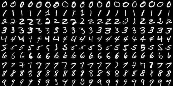
MNIST是一個非常有名的手寫體數(shù)字識別數(shù)據(jù)集，訓(xùn)練樣本：共60000個，其中55000個用于訓(xùn)練，另外5000個用于驗證；測試樣本：共10000個。MNIST數(shù)據(jù)集每張圖片是單通道的，大小為28x28。

1.1 下載并加載數(shù)據(jù)，并做出一定的預(yù)先處理

由于 MNIST 數(shù)據(jù)集圖片尺寸是 28x28 單通道的，而 LeNet-5 網(wǎng)絡(luò)輸入 Input 圖片尺寸是 32x32，因此使用 transforms.Resize 將輸入圖片尺寸調(diào)整為 32x32。

首先導(dǎo)入 PyToch 的相關(guān)算法庫：

import torchimport torch.nn as nnimport torch.nn.functional as Fimport torch.optim as optimfrom torchvision import datasets, transformsimport timefrom matplotlib import pyplot as plt

pipline_train = transforms.Compose([    #隨機旋轉(zhuǎn)圖片    transforms.RandomHorizontalFlip(),    #將圖片尺寸resize到32x32    transforms.Resize((32,32)),    #將圖片轉(zhuǎn)化為Tensor格式    transforms.ToTensor(),    #正則化(當(dāng)模型出現(xiàn)過擬合的情況時，用來降低模型的復(fù)雜度)    transforms.Normalize((0.1307,),(0.3081,))    ])pipline_test = transforms.Compose([    #將圖片尺寸resize到32x32    transforms.Resize((32,32)),    transforms.ToTensor(),    transforms.Normalize((0.1307,),(0.3081,))])#下載數(shù)據(jù)集train_set = datasets.MNIST(root="./data", train=True, download=True, transform=pipline_train)test_set = datasets.MNIST(root="./data", train=False, download=True, transform=pipline_test)#加載數(shù)據(jù)集trainloader = torch.utils.data.DataLoader(train_set, batch_size=64, shuffle=True)testloader = torch.utils.data.DataLoader(test_set, batch_size=32, shuffle=False)

這里要解釋一下 Pytorch MNIST 數(shù)據(jù)集標(biāo)準(zhǔn)化為什么是 transforms.Normalize((0.1307,), (0.3081,))？?

標(biāo)準(zhǔn)化（Normalization）是神經(jīng)網(wǎng)絡(luò)對數(shù)據(jù)的一種經(jīng)常性操作。標(biāo)準(zhǔn)化處理指的是：樣本減去它的均值，再除以它的標(biāo)準(zhǔn)差，最終樣本將呈現(xiàn)均值為 0 方差為 1 的數(shù)據(jù)分布。

神經(jīng)網(wǎng)絡(luò)模型偏愛標(biāo)準(zhǔn)化數(shù)據(jù)，原因是均值為0方差為1的數(shù)據(jù)在 sigmoid、tanh 經(jīng)過激活函數(shù)后求導(dǎo)得到的導(dǎo)數(shù)很大，反之原始數(shù)據(jù)不僅分布不均（噪聲大）而且數(shù)值通常都很大（本例中數(shù)值范圍是 0~255），激活函數(shù)后求導(dǎo)得到的導(dǎo)數(shù)則接近與 0，這也被稱為梯度消失。所以說，數(shù)據(jù)的標(biāo)準(zhǔn)化有利于加快神經(jīng)網(wǎng)絡(luò)的訓(xùn)練。?

除此之外，還需要保持 train_set、val_set 和 test_set 標(biāo)準(zhǔn)化系數(shù)的一致性。標(biāo)準(zhǔn)化系數(shù)就是計算要用到的均值和標(biāo)準(zhǔn)差，在本例中是((0.1307,), (0.3081,))，均值是 0.1307，標(biāo)準(zhǔn)差是 0.3081，這些系數(shù)都是數(shù)據(jù)集提供方計算好的數(shù)據(jù)。不同數(shù)據(jù)集就有不同的標(biāo)準(zhǔn)化系數(shù)，例如([0.485, 0.456, 0.406], [0.229, 0.224, 0.225])就是 ImageNet dataset 的標(biāo)準(zhǔn)化系數(shù)（RGB三個通道對應(yīng)三組系數(shù)），當(dāng)需要將 Imagenet 預(yù)訓(xùn)練的參數(shù)遷移到另一神經(jīng)網(wǎng)絡(luò)時，被遷移的神經(jīng)網(wǎng)絡(luò)就需要使用 Imagenet的系數(shù)，否則預(yù)訓(xùn)練不僅無法起到應(yīng)有的作用甚至還會幫倒忙。

1.2 搭建 LeNet-5 神經(jīng)網(wǎng)絡(luò)結(jié)構(gòu)，并定義前向傳播的過程

class LeNet(nn.Module):    def __init__(self):        super(LeNet, self).__init__()        self.conv1 = nn.Conv2d(1, 6, 5)         self.relu = nn.ReLU()        self.maxpool1 = nn.MaxPool2d(2, 2)        self.conv2 = nn.Conv2d(6, 16, 5)        self.maxpool2 = nn.MaxPool2d(2, 2)        self.fc1 = nn.Linear(16*5*5, 120)        self.fc2 = nn.Linear(120, 84)        self.fc3 = nn.Linear(84, 10)
    def forward(self, x):        x = self.conv1(x)        x = self.relu(x)        x = self.maxpool1(x)        x = self.conv2(x)        x = self.maxpool2(x)        x = x.view(-1, 16*5*5)        x = F.relu(self.fc1(x))        x = F.relu(self.fc2(x))        x = self.fc3(x)        output = F.log_softmax(x, dim=1)        return output

1.3 將定義好的網(wǎng)絡(luò)結(jié)構(gòu)搭載到 GPU/CPU，并定義優(yōu)化器

#創(chuàng)建模型，部署gpudevice = torch.device("cuda" if torch.cuda.is_available() else "cpu")model = LeNet().to(device)#定義優(yōu)化器optimizer = optim.Adam(model.parameters(), lr=0.001)

1.4 定義訓(xùn)練過程

def train_runner(model, device, trainloader, optimizer, epoch):    #訓(xùn)練模型, 啟用 BatchNormalization 和 Dropout, 將BatchNormalization和Dropout置為True    model.train()    total = 0    correct =0.0
    #enumerate迭代已加載的數(shù)據(jù)集,同時獲取數(shù)據(jù)和數(shù)據(jù)下標(biāo)    for i, data in enumerate(trainloader, 0):        inputs, labels = data        #把模型部署到device上        inputs, labels = inputs.to(device), labels.to(device)        #初始化梯度        optimizer.zero_grad()        #保存訓(xùn)練結(jié)果        outputs = model(inputs)        #計算損失和        #多分類情況通常使用cross_entropy(交叉熵?fù)p失函數(shù)), 而對于二分類問題, 通常使用sigmod        loss = F.cross_entropy(outputs, labels)        #獲取最大概率的預(yù)測結(jié)果        #dim=1表示返回每一行的最大值對應(yīng)的列下標(biāo)        predict = outputs.argmax(dim=1)        total += labels.size(0)        correct += (predict == labels).sum().item()        #反向傳播        loss.backward()        #更新參數(shù)        optimizer.step()        if i % 1000 == 0:            #loss.item()表示當(dāng)前l(fā)oss的數(shù)值            print("Train Epoch{} \t Loss: {:.6f}, accuracy: {:.6f}%".format(epoch, loss.item(), 100*(correct/total)))            Loss.append(loss.item())            Accuracy.append(correct/total)    return loss.item(), correct/total

1.5 定義測試過程

def test_runner(model, device, testloader):    #模型驗證, 必須要寫, 否則只要有輸入數(shù)據(jù), 即使不訓(xùn)練, 它也會改變權(quán)值    #因為調(diào)用eval()將不啟用 BatchNormalization 和 Dropout, BatchNormalization和Dropout置為False    model.eval()    #統(tǒng)計模型正確率, 設(shè)置初始值    correct = 0.0    test_loss = 0.0    total = 0    #torch.no_grad將不會計算梯度, 也不會進(jìn)行反向傳播    with torch.no_grad():        for data, label in testloader:            data, label = data.to(device), label.to(device)            output = model(data)            test_loss += F.cross_entropy(output, label).item()            predict = output.argmax(dim=1)            #計算正確數(shù)量            total += label.size(0)            correct += (predict == label).sum().item()        #計算損失值        print("test_avarage_loss: {:.6f}, accuracy: {:.6f}%".format(test_loss/total, 100*(correct/total)))

1.6 運行

LeNet-5 網(wǎng)絡(luò)模型定義好，訓(xùn)練函數(shù)、驗證函數(shù)也定義好了，就可以直接使用 MNIST 數(shù)據(jù)集進(jìn)行訓(xùn)練了。

# 調(diào)用epoch = 5Loss = []Accuracy = []for epoch in range(1, epoch+1):    print("start_time",time.strftime('%Y-%m-%d %H:%M:%S',time.localtime(time.time())))    loss, acc = train_runner(model, device, trainloader, optimizer, epoch)    Loss.append(loss)    Accuracy.append(acc)    test_runner(model, device, testloader)    print("end_time: ",time.strftime('%Y-%m-%d %H:%M:%S',time.localtime(time.time())),'\n')
print('Finished Training')plt.subplot(2,1,1)plt.plot(Loss)plt.title('Loss')plt.show()plt.subplot(2,1,2)plt.plot(Accuracy)plt.title('Accuracy')plt.show()

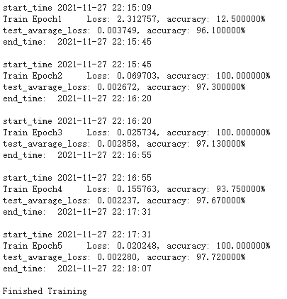
經(jīng)歷 5 次 epoch 的 loss 和 accuracy 曲線如下：

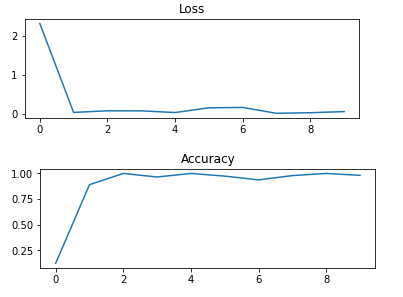
最終在 10000 張測試樣本上，average_loss降到了?0.00228，accuracy 達(dá)到了 97.72%。可以說 LeNet-5 的效果非常好！

1.7 保存模型

print(model)torch.save(model, './models/model-mnist.pth') #保存模型

LeNet-5 的模型會 print 出來，并將模型模型命令為 model-mnist.pth 保存在固定目錄下。

LeNet(
  (conv1): Conv2d(1, 6, kernel_size=(5, 5), stride=(1, 1))
  (relu): ReLU()
  (maxpool1): MaxPool2d(kernel_size=2, stride=2, padding=0, dilation=1, ceil_mode=False)
  (conv2): Conv2d(6, 16, kernel_size=(5, 5), stride=(1, 1))
  (maxpool2): MaxPool2d(kernel_size=2, stride=2, padding=0, dilation=1, ceil_mode=False)
  (fc1): Linear(in_features=400, out_features=120, bias=True)
  (fc2): Linear(in_features=120, out_features=84, bias=True)
  (fc3): Linear(in_features=84, out_features=10, bias=True)
)

1.8 手寫圖片的測試

下面，我們將利用剛剛訓(xùn)練的 LeNet-5 模型進(jìn)行手寫數(shù)字圖片的測試。

import cv2
if __name__ == '__main__':    device = torch.device('cuda' if torch.cuda.is_available() else 'cpu')    model = torch.load('./models/model-mnist.pth') #加載模型    model = model.to(device)    model.eval()    #把模型轉(zhuǎn)為test模式
    #讀取要預(yù)測的圖片    img = cv2.imread("./images/test_mnist.jpg")    img=cv2.resize(img,dsize=(32,32),interpolation=cv2.INTER_NEAREST)    plt.imshow(img,cmap="gray") # 顯示圖片    plt.axis('off') # 不顯示坐標(biāo)軸    plt.show()
    # 導(dǎo)入圖片，圖片擴展后為[1，1，32，32]    trans = transforms.Compose(        [            transforms.ToTensor(),            transforms.Normalize((0.1307,), (0.3081,))        ])    img = cv2.cvtColor(img, cv2.COLOR_BGR2GRAY)#圖片轉(zhuǎn)為灰度圖，因為mnist數(shù)據(jù)集都是灰度圖    img = trans(img)    img = img.to(device)????img?=?img.unsqueeze(0)??#圖片擴展多一維,因為輸入到保存的模型中是4維的[batch_size,通道,長，寬]，而普通圖片只有三維，[通道,長，寬]????    # 預(yù)測     output = model(img)    prob = F.softmax(output,dim=1) #prob是10個分類的概率    print("概率：",prob)    value, predicted = torch.max(output.data, 1)    predict = output.argmax(dim=1)    print("預(yù)測類別：",predict.item())

輸出：

概率：tensor([[2.0888e-07, 1.1599e-07, 6.1852e-05, 1.5797e-04, 1.4975e-09, 9.9977e-01,
? ? ? ? 1.9271e-06, 3.1589e-06, 1.2186e-07, 4.3405e-07]],
? ? ? grad_fn=)
預(yù)測類別：5

模型預(yù)測結(jié)果正確！

以上就是 PyTorch 構(gòu)建 LeNet-5 卷積神經(jīng)網(wǎng)絡(luò)并用它來識別 MNIST 數(shù)據(jù)集的例子。全文的代碼都是可以順利運行的，建議大家自己跑一邊。

所有完整的代碼我都放在 GitHub 上，GitHub地址為：

https://github.com/RedstoneWill/ObjectDetectionLearner/tree/main/LeNet-5

也可以點擊閱讀原文進(jìn)入~


往期精彩回顧




適合初學(xué)者入門人工智能的路線及資料下載
中國大學(xué)慕課《機器學(xué)習(xí)》（黃海廣主講）
機器學(xué)習(xí)及深度學(xué)習(xí)筆記等資料打印
機器學(xué)習(xí)在線手冊
深度學(xué)習(xí)筆記專輯
《統(tǒng)計學(xué)習(xí)方法》的代碼復(fù)現(xiàn)專輯
AI基礎(chǔ)下載
本站qq群955171419，加入微信群請掃碼：

【深度學(xué)習(xí)】我用 PyTorch 復(fù)現(xiàn)了 LeNet-5 神經(jīng)網(wǎng)絡(luò)（MNIST 手寫數(shù)據(jù)集篇）！

一、使用 LeNet-5 網(wǎng)絡(luò)結(jié)構(gòu)創(chuàng)建 MNIST 手寫數(shù)字識別分類器