引言

本著“凡我不能創(chuàng)造的，我就不能理解”的思想，本系列文章會(huì)基于純Python以及NumPy從零創(chuàng)建自己的深度學(xué)習(xí)框架，該框架類似PyTorch能實(shí)現(xiàn)自動(dòng)求導(dǎo)。

要深入理解深度學(xué)習(xí)，從零開始創(chuàng)建的經(jīng)驗(yàn)非常重要，從自己可以理解的角度出發(fā)，盡量不適用外部完備的框架前提下，實(shí)現(xiàn)我們想要的模型。本系列文章的宗旨就是通過這樣的過程，讓大家切實(shí)掌握深度學(xué)習(xí)底層實(shí)現(xiàn)，而不是僅做一個(gè)調(diào)包俠。

上篇文章對(duì)Softmax邏輯回歸進(jìn)行了簡(jiǎn)單的介紹，本文我們就來(lái)從零實(shí)現(xiàn)Softmax邏輯回歸。

實(shí)現(xiàn)Softmax函數(shù)

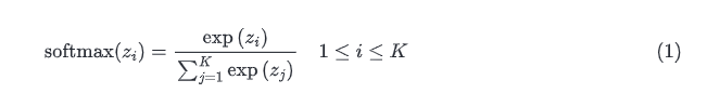
首先我們實(shí)現(xiàn)Softmax回歸的靈魂：

def?softmax(x,?axis=-1):
????y?=?x.exp()
????return?y?/?y.sum(axis=axis,?keepdims=True)

實(shí)現(xiàn)交叉熵?fù)p失函數(shù)

def?cross_entropy(input:?Tensor,?target:?Tensor,?reduction:?str?=?"mean")?->?Tensor:
????N?=?len(target)

????p?=?softmax(input)

????errors?=?-?target?*?p.log()
????#?errors?=?-?p[np.arange(N),?target.data].log()

????if?reduction?==?"mean":
????????loss?=?errors.sum()?/?N
????elif?reduction?==?"sum":
????????loss?=?errors.sum()
????else:
????????loss?=?errors
????return?loss

這里調(diào)用剛才實(shí)現(xiàn)的softmax函數(shù)把輸入input轉(zhuǎn)換成概率，所以這里的輸入實(shí)際上是logits，即未經(jīng)過Softmax的值。

然后我們基于此實(shí)現(xiàn)損失類：

class?CrossEntropyLoss(_Loss):
????def?__init__(self,?reduction:?str?=?"mean")?->?None:
????????super().__init__(reduction)

????def?forward(self,?input:?Tensor,?target:?Tensor)?->?Tensor:
????????return?F.cross_entropy(input,?target,?self.reduction)

實(shí)現(xiàn)Softmax回歸

class?SoftmaxRegression(Module):
????def?__init__(self,?input_dim,?output_dim):
????????self.linear?=?Linear(input_dim,?output_dim)

????def?forward(self,?x:?Tensor)?->?Tensor:
????????#?只要輸出logits即可
????????return?self.linear(x)

這里只需要計(jì)算出的結(jié)果即可。

使用Softmax回歸分類鳶尾花

我們加載sklearn中的iris數(shù)據(jù)集。

鳶尾花如上所示，有4個(gè)特征：

• Sepal.Length（花萼長(zhǎng)度）

• Sepal.Width（花萼寬度）

• Petal.Length（花瓣長(zhǎng)度）

• Petal.Width（花瓣寬度）

有三個(gè)類別：Iris Setosa（山鳶尾）、Iris Versicolour（雜色鳶尾），以及Iris Virginica（維吉尼亞鳶尾）。

為了可視化的方便，我們先只考慮兩個(gè)特征，可視化結(jié)果如下：

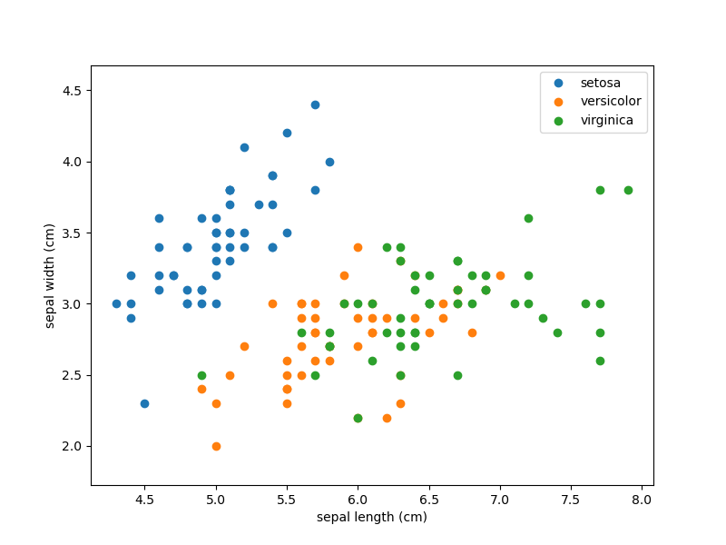
從上圖可以看到，只考慮前兩個(gè)特征的情況下，橙色店和綠色點(diǎn)看起來(lái)不太好分，這暫且不管，我們先寫代碼，硬Train一發(fā)。

def?generate_dataset(draw_picture=False):
????iris?=?datasets.load_iris()

????X?=?iris['data'][:,?:2]??#?我們只需要前兩個(gè)特征
????y?=?iris['target']
????names?=?iris['target_names']??#?類名
????feature_names?=?iris['feature_names']??#?特征名

????if?draw_picture:
????????x_min,?x_max?=?X[:,?0].min()?-?0.5,?X[:,?0].max()?+?0.5
????????y_min,?y_max?=?X[:,?1].min()?-?0.5,?X[:,?1].max()?+?0.5

????????plt.figure(2,?figsize=(8,?6))
????????plt.clf()

????????for?target,?target_name?in?enumerate(names):
????????????X_plot?=?X[y?==?target]
????????????plt.plot(X_plot[:,?0],?X_plot[:,?1],
?????????????????????linestyle='none',
?????????????????????marker='o',
?????????????????????label=target_name)
????????plt.xlabel(feature_names[0])
????????plt.ylabel(feature_names[1])
????????plt.xlim(x_min,?x_max)
????????plt.ylim(y_min,?y_max)

????????plt.axis('equal')
????????plt.legend()

????????fig?=?plt.gcf()
????????fig.savefig('iris.png',?dpi=100)

????y?=?np.eye(3)[y]

????X_train,?X_test,?y_train,?y_test?=?train_test_split(
????????X,?y,?test_size=0.2,?random_state=2)

????return?Tensor(X_train),?Tensor(X_test),?Tensor(y_train),?Tensor(y_test)


if?__name__?==?'__main__':
????X_train,?X_test,?y_train,?y_test?=?generate_dataset(True)
????epochs?=?2000

????model?=?SoftmaxRegression(2,?3)??#?2個(gè)特征?3個(gè)輸出

????optimizer?=?SGD(model.parameters(),?lr=1e-1)

????loss?=?CrossEntropyLoss()

????losses?=?[]

????for?epoch?in?range(int(epochs)):
????????outputs?=?model(X_train)
????????l?=?loss(outputs,?y_train)
????????optimizer.zero_grad()
????????l.backward()
????????optimizer.step()

????????if?(epoch?+?1)?%?20?==?0:
????????????losses.append(l.item())
????????????print(f"Train?-??Loss:?{l.item()}")

????#?在測(cè)試集上測(cè)試
????outputs?=?model(X_test)
????correct?=?np.sum(outputs.numpy().argmax(-1)?==?y_test.numpy().argmax(-1))
????accuracy?=?100?*?correct?/?len(y_test)
????print(f"Test?Accuracy:{accuracy}")

為了驗(yàn)證泛化能力，我們這里還區(qū)分了訓(xùn)練集和測(cè)試集。

Train?-??Loss:?0.9068448543548584
Train?-??Loss:?0.8322725296020508
Train?-??Loss:?0.7793639302253723
Train?-??Loss:?0.740231454372406
...
Train?-??Loss:?0.4532046616077423
Train?-??Loss:?0.45260095596313477
Train?-??Loss:?0.45200586318969727
Train?-??Loss:?0.45141926407814026
Train?-??Loss:?0.45084092020988464
Train?-??Loss:?0.4502706527709961
Train?-??Loss:?0.44970834255218506
Train?-??Loss:?0.4491537809371948
Train?-??Loss:?0.44860681891441345
Test?Accuracy:76.66666666666667

如果我們考慮所有的特征準(zhǔn)確率會(huì)不會(huì)很一點(diǎn)？

我們只要修改兩行代碼：

def?generate_dataset(draw_picture=False):
????iris?=?datasets.load_iris()

????X?=?iris['data']?#?修改這里
????
#?修改模型的參數(shù)
model?=?SoftmaxRegression(4,?3)??#?4個(gè)特征?3個(gè)輸出

再次訓(xùn)練查看結(jié)果：

Train?-??Loss:?0.7530185580253601
Train?-??Loss:?0.6372731328010559
Train?-??Loss:?0.5648812055587769
Train?-??Loss:?0.5048649907112122
Train?-??Loss:?0.44937923550605774
Train?-??Loss:?0.3961796164512634
Train?-??Loss:?0.3457953631877899
Train?-??Loss:?0.3021572232246399
Train?-??Loss:?0.27336016297340393
...
Train?-??Loss:?0.09917300194501877
Train?-??Loss:?0.09881455451250076
Train?-??Loss:?0.09846225380897522
Train?-??Loss:?0.0981159582734108
Train?-??Loss:?0.09777550399303436
Test?Accuracy:100.0

啥也不說了。

完整代碼

完整代碼筆者上傳到了程序員最大交友網(wǎng)站上去了，地址: [?? ?https://github.com/nlp-greyfoss/metagrad]

總結(jié)

本文我們實(shí)現(xiàn)了能支持多個(gè)類別的多元邏輯回歸，并且看到了在模型中充分利用已有的特征是有多重要。