午夜精品18 视频国产,国产色婷婷国产综合在线,天天爽天天操,日韩免费黄,91中文字幕网,国产99在线,亚洲无码国产乱伦,国产1区2区3区

關(guān)于對抗生成網(wǎng)絡(luò)的概念，前面已經(jīng)說了不少了，話不多說，直接開整！

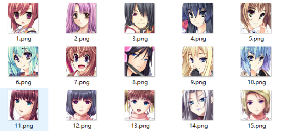
我們的數(shù)據(jù)集如下（共2.1w+張圖片,回復(fù)“動漫人臉”即可獲取下載鏈接）：

數(shù)據(jù)加載

DataSets

接著，我們加載這些二次元頭像，然后進(jìn)行數(shù)據(jù)處理，新建一個dcgan.py文件寫入如下代碼：

主要的作用是把圖片加載進(jìn)內(nèi)存，內(nèi)存比較小的同學(xué)可以將它改寫成生成器的方式。

import tensorflow.keras as kerasfrom tensorflow.keras import layersimport numpy as npimport osimport cv2from tensorflow.keras.preprocessing import imageimport mathfrom PIL import Image
anime_path = './amine'
# 導(dǎo)入數(shù)據(jù)集x_train = []for i in os.listdir(anime_path):    image_path = os.path.join(anime_path, i)    img = cv2.imread(image_path)    img = cv2.cvtColor(img, cv2.COLOR_BGR2RGB)    x_train.append(img)
# 數(shù)據(jù)集處理x_train = np.array(x_train)x_train = x_train.reshape(-1, 64, 64, 3)print(x_train.shape)

模型搭建

Model

接著，我們搭建網(wǎng)絡(luò)模型，我們知道，生成對抗網(wǎng)絡(luò)是由2個模型相互對抗得到的，所以在這里我們需要搭建2個網(wǎng)絡(luò)，分別是生成網(wǎng)絡(luò)和判別網(wǎng)絡(luò)：

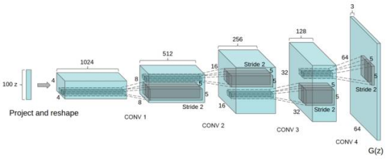
生成網(wǎng)絡(luò)的結(jié)構(gòu)大體如下，我們可以看到，生成網(wǎng)絡(luò)的輸入是一個長度為100的噪聲，接著與一個4*4*1024的特征向量做全連接，然后使用反卷積一步一步進(jìn)行上采樣，最后得到一張64*64*3的圖片：

我們對這個網(wǎng)絡(luò)進(jìn)行稍微的修改，代碼如下

# 定義網(wǎng)絡(luò)參數(shù)latent_dim = 64 # 輸入生成網(wǎng)絡(luò)的噪聲height = 64width = 64channels = 3
generator_input = keras.Input(shape=(latent_dim,))# 首先，將輸入轉(zhuǎn)換為16 x 16 x 256通道的feature mapx = layers.Dense(256 * 16 * 16)(generator_input)x = layers.LeakyReLU()(x)x = layers.Reshape((16, 16, 256))(x)# 然后，添加卷積層x = layers.Conv2D(128, 5, padding='same')(x)x = layers.LeakyReLU()(x)# 上采樣至 32 x 32x = layers.Conv2DTranspose(128, 5, strides=2, padding='same')(x)x = layers.LeakyReLU()(x)# 上采樣至 64 x 64x = layers.Conv2DTranspose(128, 5, strides=2, padding='same')(x)x = layers.LeakyReLU()(x)# 添加更多的卷積層x = layers.Conv2D(64, 5, padding='same')(x)x = layers.LeakyReLU()(x)# 生成一個 64 x 64 1-channel 的feature mapx = layers.Conv2D(channels, 7, activation='tanh', padding='same')(x)generator = keras.models.Model(generator_input, x)generator.summary()

接著，我們搭建判別網(wǎng)絡(luò)，判別網(wǎng)絡(luò)其實和普通的圖片分類網(wǎng)絡(luò)沒什么區(qū)別，輸入是一張64*64*3的圖片，經(jīng)過一系列的卷積和下采樣，最終得到分類結(jié)果。

判別網(wǎng)絡(luò)代碼如下：

discriminator_input = layers.Input(shape=(height, width, channels))x = layers.Conv2D(256, 3)(discriminator_input)x = layers.LeakyReLU()(x)
x = layers.Conv2D(256, 3, strides=2)(x)x = layers.LeakyReLU()(x)
x = layers.Conv2D(128, 3, strides=2)(x)x = layers.LeakyReLU()(x)
x = layers.Conv2D(128, 3, strides=2)(x)x = layers.LeakyReLU()(x)x = layers.Flatten()(x)# 重要的技巧(添加一個dropout層)x = layers.Dropout(0.3)(x)# 分類層x = layers.Dense(1, activation='sigmoid')(x)discriminator = keras.models.Model(discriminator_input, x)keras.utils.plot_model(discriminator, 'dis.png', show_shapes=True)discriminator.summary()

我們對比以上兩個網(wǎng)絡(luò)，會發(fā)現(xiàn)一個有趣的問題，這兩個網(wǎng)絡(luò)其實是相反的，生成網(wǎng)絡(luò)是給定一組噪聲，通過上采樣生成一張圖片，而判別網(wǎng)絡(luò)是給定一張圖片，通過下采樣生成概率。

接著我們編譯判別器網(wǎng)絡(luò)，并設(shè)置判別器為不訓(xùn)練狀態(tài)，然后組裝GAN網(wǎng)絡(luò)：

optimizer = keras.optimizers.Adam(0.0002, 0.5)# 編譯判斷器網(wǎng)絡(luò)discriminator_optimizer = keras.optimizers.RMSprop(lr=8e-4, clipvalue=1.0, decay=1e-8)discriminator.compile(optimizer=optimizer, loss='binary_crossentropy')
# 設(shè)置判別器為不訓(xùn)練(單獨交替迭代訓(xùn)練)discriminator.trainable = False# 組裝GAN網(wǎng)絡(luò)gan_input = keras.Input(shape=(latent_dim,))gan_output = discriminator(generator(gan_input))gan = keras.models.Model(gan_input, gan_output)
gan_optimizer = keras.optimizers.Adam(lr=4e-4, clipvalue=1.0, decay=1e-8)gan.compile(optimizer=optimizer, loss='binary_crossentropy')

GAN網(wǎng)絡(luò)的運作流程如下：1.輸入一個長度為100的噪聲，通過生成網(wǎng)絡(luò)生成一張圖片。2.將生成網(wǎng)絡(luò)生成的圖片送入判別網(wǎng)絡(luò)中，得到判別結(jié)果。3.在這個過程中，需要平衡生成器與判別器，所以將判別網(wǎng)絡(luò)設(shè)置為不訓(xùn)練狀態(tài)。網(wǎng)絡(luò)形如：

開始訓(xùn)練

Train

完成了這些，其實我們就可以開始訓(xùn)練函數(shù)的編寫了，但是為了后面更好地觀看生成的圖片，我們再寫一個組合圖片的函數(shù)

# 將一個批次的圖片合成一張圖片def combine_images(generated_images):    '''    :param generated_images: 一個批次的圖片    :return: 圖片    '''    num = generated_images.shape[0] # 圖片的數(shù)量(-1, 64, 64, 3)    width = int(math.sqrt(num))     # 新創(chuàng)建圖片的寬度    height = int(math.ceil(float(num) / width))    shape = generated_images.shape[1:3]    # 生成一張純黑色圖片    image = np.zeros((height * shape[0], width * shape[1], 3),                     dtype=generated_images.dtype)    # 循環(huán)每張圖片，并將圖片內(nèi)的像素點填充到生成的黑色圖片中    for index, img in enumerate(generated_images):        i = int(index / width)        j = index % width        # 分別填充3個通道        image[i * shape[0]:(i+1) * shape[0], j * shape[1]:(j+1) * shape[1], 0] = \            img[:, :, 0]        image[i * shape[0]:(i+1) * shape[0], j * shape[1]:(j+1) * shape[1], 1] = \            img[:, :, 1]        image[i * shape[0]:(i+1) * shape[0], j * shape[1]:(j+1) * shape[1], 2] = \            img[:, :, 2]    return image

接著定義訓(xùn)練參數(shù)：

# 歸一化x_train = x_train.astype('float32') / 255.iterations = 50000batch_size = 16start = 0save_dir = './save'

然后使用for循環(huán)開始訓(xùn)練，在每一個批次的訓(xùn)練中，我們需要生成隨機點送入生成器生成假圖像，然后將假圖像和真圖像進(jìn)行比較，并組合標(biāo)簽，然后單獨訓(xùn)練判別器，接著訓(xùn)練GAN網(wǎng)絡(luò)，這時候判別器的權(quán)重被凍結(jié)。最后我們每隔一定的周期保存好模型與生成的圖片，便于觀察生成器的效果

for step in range(iterations):    # 在潛在空間中抽樣隨機點    random_latent_vectors = np.random.normal(size=(batch_size, latent_dim))    # print(random_latent_vecotors.shape)    # 將隨機抽樣點解碼為假圖像    generated_images = generator.predict(random_latent_vectors)
    # 將假圖像與真實圖像進(jìn)行比較    stop = start + batch_size    real_images = x_train[start: stop]    combined_images = np.concatenate([generated_images, real_images])
    # 組裝區(qū)別真假圖像的標(biāo)簽（真全為1 假全為0）    labels = np.concatenate([np.ones((batch_size, 1)),                             np.zeros((batch_size, 1))])    # 重要的技巧，在標(biāo)簽上添加隨機噪聲    labels += 0.05 * np.random.random(labels.shape)    # 訓(xùn)練鑒別器（discrimitor）    d_loss = discriminator.train_on_batch(combined_images, labels)    # 在潛在空間中采樣隨機點    random_latent_vectors = np.random.normal(size=(batch_size, latent_dim))
    # 匯集標(biāo)有“所有真實圖像”的標(biāo)簽    misleading_targets = np.zeros((batch_size, 1))
    # 訓(xùn)練生成器（generator） （通過gan模型，鑒別器（discrimitor）權(quán)值被凍結(jié)）    a_loss = gan.train_on_batch(random_latent_vectors, misleading_targets)
    start += batch_size    if start > len(x_train) - batch_size:        start = 0
    if step % 500 == 0:        gan.save('gan.h5')        generator.save('generator.h5')        print('step: %s, d_loss: %s, a_loss: %s' % (step, d_loss, a_loss))        # 保存生成的圖像        img = combine_images(generated_images)  # 組合圖片        img = image.array_to_img(img * 255., scale=False)        img.save(save_dir + '/anime_' + str(step) + '.png')

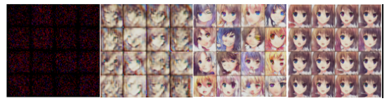
最后，我們就可以右鍵運行程序了，GAN訓(xùn)練的時候需要大量的時間，所以要耐心等待！放幾張圖片感受一下:

測試

Test

在上面的訓(xùn)練中，我們一邊訓(xùn)練一邊保存了模型的權(quán)重，在使用的時候，我們只需要加載保存后的生成網(wǎng)絡(luò)的權(quán)重即可進(jìn)行測試：

import tensorflow.keras as kimport numpy as npimport matplotlib.pyplot as pltfrom  tensorflow.keras.preprocessing import image
#加載模型model=k.models.load_model('generator.h5')model.summary()
#生成0~1的隨機噪聲random_latent_vectors = np.random.uniform(0,1,size=(1, 64))print(random_latent_vectors)
#*255random_latent_vectors=random_latent_vectors*255.#轉(zhuǎn)換成unit8格式random_latent_vectors.astype('uint8')plt.axis('off')plt.imshow(random_latent_vectors)#放入模型中預(yù)測generated_images = model.predict(random_latent_vectors)#數(shù)組轉(zhuǎn)圖片格式img = image.array_to_img(generated_images[0]* 255., scale=False)plt.imshow(img)

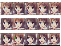
運行結(jié)果如下：

掃二維碼｜關(guān)注我們

微信號｜深度學(xué)習(xí)從入門到放棄

長按關(guān)注｜永不迷路

有趣的對抗生成網(wǎng)絡(luò)（六）二次元頭像生成