
【機(jī)器學(xué)習(xí)】三大樹模型實(shí)戰(zhàn)乳腺癌預(yù)測(cè)分類
公眾號(hào):尤而小屋
作者:Peter
編輯:Peter
今天給大家?guī)?lái)一篇新的UCI數(shù)據(jù)集建模的文章。
本文從數(shù)據(jù)的探索分析出發(fā),經(jīng)過(guò)特征工程和樣本均衡性處理,使用決策樹、隨機(jī)森林、梯度提升樹對(duì)一份女性乳腺癌的數(shù)據(jù)集進(jìn)行分析和預(yù)測(cè)建模。
關(guān)鍵詞:相關(guān)性、決策樹、隨機(jī)森林、降維、獨(dú)熱碼、乳腺癌

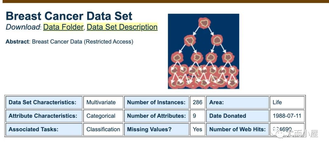
數(shù)據(jù)集
數(shù)據(jù)是來(lái)自UCI官網(wǎng),很老的一份數(shù)據(jù),主要是用于分類問(wèn)題,可以自行下載學(xué)習(xí)
https://archive.ics.uci.edu/ml/datasets/breast+cancer
導(dǎo)入庫(kù)
import?pandas?as?pd
import?numpy?as?np

import?matplotlib.pyplot?as?plt
import?seaborn?as?sns
%matplotlib?inline

import?plotly_express?as?px
import?plotly.graph_objects?as?go

from?sklearn.ensemble?import?RandomForestClassifier
from?sklearn.tree?import?DecisionTreeClassifier

from?sklearn.tree?import?export_graphviz
from?sklearn.metrics?import?roc_curve,?auc
from?sklearn.metrics?import?classification_report
from?sklearn.metrics?import?confusion_matrix
from?sklearn?import?metrics?

from?sklearn.model_selection?import?train_test_split
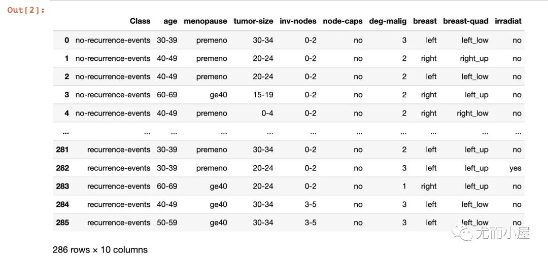
導(dǎo)入數(shù)據(jù)
數(shù)據(jù)是來(lái)自UCI官網(wǎng),下載到本地可以直接讀取。只是這份數(shù)據(jù)是.data文件,沒(méi)有文件頭,我們需要自行指定對(duì)應(yīng)的文件頭(網(wǎng)上搜索的)
#?來(lái)自u(píng)ci

df?=?pd.read_table("breast-cancer.data",
???????????????????sep=",",
???????????????????names=["Class","age","menopause","tumor-size","inv-nodes",
??????????????????????????"node-caps","deg-malig","breast","breast-quad","irradiat"])

df
基本信息
In [3]:
df.dtypes???#?字段類型
Out[3]:
全部是object類型,只有一個(gè)int64類型
Class??????????object
age????????????object
menopause??????object
tumor-size?????object
inv-nodes??????object
node-caps??????object
deg-malig???????int64
breast?????????object
breast-quad????object
irradiat???????object
dtype:?object
In [4]:
df.isnull().sum()??#?缺失值
Out[4]:
數(shù)據(jù)比較完整,沒(méi)有缺失值
Class??????????0
age????????????0
menopause??????0
tumor-size?????0
inv-nodes??????0
node-caps??????0
deg-malig??????0
breast?????????0
breast-quad????0
irradiat???????0
dtype:?int64
In [5]:
##?字段解釋

columns?=?df.columns.tolist()
columns
Out[5]:
['Class',
?'age',
?'menopause',
?'tumor-size',
?'inv-nodes',
?'node-caps',
?'deg-malig',
?'breast',
?'breast-quad',
?'irradiat']
下面是每個(gè)字段的含義和具體的取值范圍:
| 屬性名 | 含義 | 取值范圍 |
|---|---|---|
| Class | 是否復(fù)發(fā) | no-recurrence-events, recurrence-events |
| age | 年齡 | 10-19, 20-29, 30-39, 40-49, 50-59, 60-69, 70-79, 80-89, 90-99 |
| menopause | 絕經(jīng)情況 | lt40(40歲之前絕經(jīng)), ge40(40歲之后絕經(jīng)), premeno(還未絕經(jīng)) |
| tumor-size | 腫瘤大小 | 0-4, 5-9, 10-14, 15-19, 20-24, 25-29, 30-34, 35-39, 40-44, 45-49, 50-54, 55-59 |
| inv-nodes | 受侵淋巴結(jié)數(shù) | 0-2, 3-5, 6-8, 9-11, 12-14, 15-17, 18-20, 21-23, 24-26, 27-29, 30-32, 33-35, 36-39 |
| node-caps | 有無(wú)結(jié)節(jié)帽 | yes, no |
| deg-malig | 惡性腫瘤程度 | 1, 2, 3 |
| breast | 腫塊位置 | left, right |
| breast-quad | 腫塊所在象限 | left-up, left-low, right-up, right-low, central |
| irradiat | 是否放療 | yes,no |
去除缺失值
In [6]:
兩個(gè)字段中的?就是本數(shù)據(jù)中的缺失值,我們直接選擇非缺失值值的數(shù)據(jù)
df?=?df[(df["node-caps"]?!=?"?")?&?(df["breast-quad"]?!=?"?")]

len(df)
Out[6]:
277
字段處理
In [7]:
from?sklearn.preprocessing?import?LabelEncoder
年齡段-age
In [8]:
age?=?df["age"].value_counts().reset_index()
age.columns?=?["年齡段",?"人數(shù)"]

age

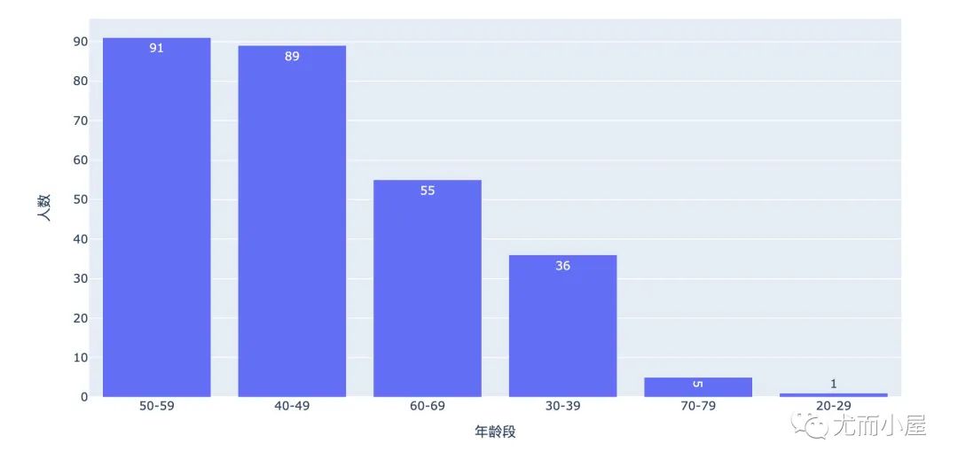
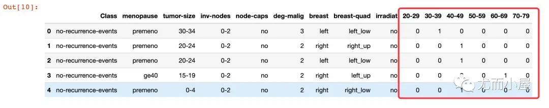
可以看到數(shù)據(jù)中大部分的用戶集中在40-59歲。對(duì)年齡段執(zhí)行獨(dú)熱碼:
df?=?df.join(pd.get_dummies(df["age"]))
df.drop("age",?axis=1,?inplace=True)
df.head()
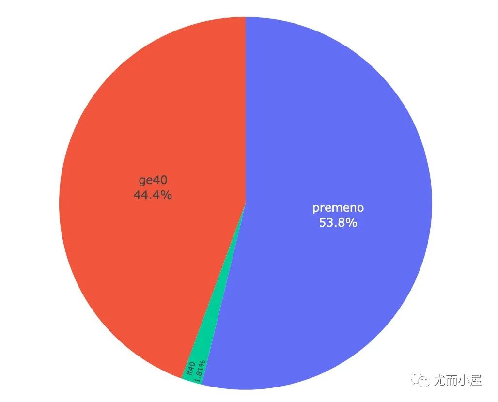
絕經(jīng)-menopause
In [11]:
menopause?=?df["menopause"].value_counts().reset_index()
menopause
Out[11]:
| index | menopause | |
|---|---|---|
| 0 | premeno | 149 |
| 1 | ge40 | 123 |
| 2 | lt40 | 5 |
In [12]:
fig?=?px.pie(menopause,names="index",values="menopause")

fig.update_traces(
????textposition='inside',???
????textinfo='percent+label')

fig.show()
df?=?df.join(pd.get_dummies(df["menopause"]))??#?獨(dú)熱碼

df.drop("menopause",axis=1,?inplace=True)
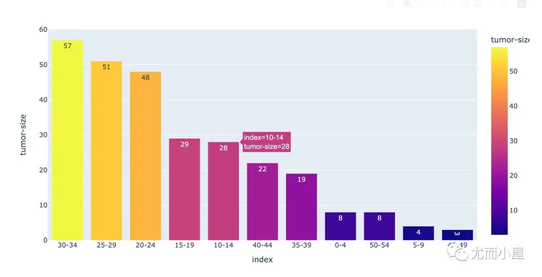
腫瘤大小-tumor-size
In [14]:
tumor_size?=?df["tumor-size"].value_counts().reset_index()

tumor_size
Out[14]:
| index | tumor-size | |
|---|---|---|
| 0 | 30-34 | 57 |
| 1 | 25-29 | 51 |
| 2 | 20-24 | 48 |
| 3 | 15-19 | 29 |
| 4 | 10-14 | 28 |
| 5 | 40-44 | 22 |
| 6 | 35-39 | 19 |
| 7 | 0-4 | 8 |
| 8 | 50-54 | 8 |
| 9 | 5-9 | 4 |
| 10 | 45-49 | 3 |
In [15]:
fig?=?px.bar(tumor_size,?
?????????????x="index",
?????????????y="tumor-size",
?????????????color="tumor-size",
?????????????text="tumor-size")

fig.show()
df?=?df.join(pd.get_dummies(df["tumor-size"]))

df.drop("tumor-size",axis=1,?inplace=True)
In [18]:
df?=?df.join(pd.get_dummies(df["inv-nodes"]))

df.drop("inv-nodes",axis=1,?inplace=True)
有無(wú)結(jié)節(jié)帽-node-caps
In [19]:
df["node-caps"].value_counts()
Out[19]:
no?????221
yes?????56
Name:?node-caps,?dtype:?int64
In [20]:
df?=?df.join(pd.get_dummies(df["node-caps"]).rename(columns={"no":"node_capes_no",?"yes":"node_capes_yes"}))

df.drop("node-caps",axis=1,?inplace=True)
惡性腫瘤程度-deg-malig
In [21]:
df["deg-malig"].value_counts()
Out[21]:
2????129
3?????82
1?????66
Name:?deg-malig,?dtype:?int64
腫塊位置-breast
In [22]:
df["breast"].value_counts()
Out[22]:
left?????145
right????132
Name:?breast,?dtype:?int64
In [23]:
df?=?df.join(pd.get_dummies(df["breast"]))

df.drop("breast",axis=1,?inplace=True)
...
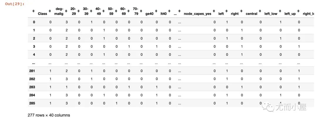
是否復(fù)發(fā)-Class
這個(gè)是最終預(yù)測(cè)的因變量,我們需要將文本信息轉(zhuǎn)成0-1的數(shù)值信息
In [29]:
dic?=?{"no-recurrence-events":0,?"recurrence-events":1}
df["Class"]?=?df["Class"].map(dic)??#?實(shí)施轉(zhuǎn)換

df
復(fù)發(fā)和非復(fù)發(fā)的統(tǒng)計(jì):
sns.countplot(df['Class'],label="Count")

plt.show()
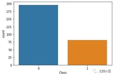
樣本不均衡處理
In [31]:
#?樣本量分布

df["Class"].value_counts()
Out[31]:
0????196
1?????81
Name:?Class,?dtype:?int64
In [32]:
from?imblearn.over_sampling?import?SMOTE
In [33]:
X?=?df.iloc[:,1:]
y?=?df.iloc[:,0]

y.head()
Out[33]:
0????0
1????0
2????0
3????0
4????0
Name:?Class,?dtype:?int64
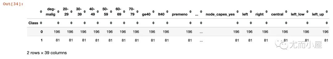
In [34]:
groupby_df?=?df.groupby('Class').count()??????

#?輸出原始數(shù)據(jù)集樣本分類分布
groupby_df
model_smote?=?SMOTE()

x_smote_resampled,?y_smote_resampled?=?model_smote.fit_resample(X,?y)?????????
x_smoted?=?pd.DataFrame(x_smote_resampled,?
????????????????????????columns=df.columns.tolist()[1:])???
y_smoted?=?pd.DataFrame(y_smote_resampled,
????????????????????????columns=['Class'])???????
df_smoted?=?pd.concat([x_smoted,?y_smoted],axis=1)
建模
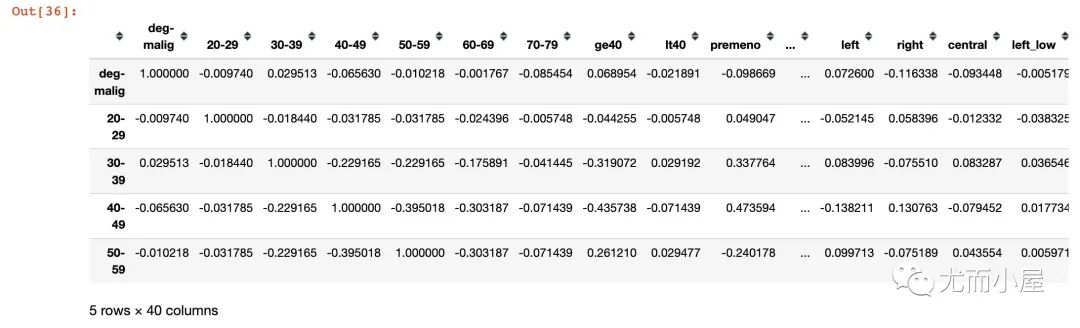
相關(guān)性
分析每個(gè)新字段和因變量之間的相關(guān)性
In [36]:
corr?=?df_smoted.corr()
corr.head()
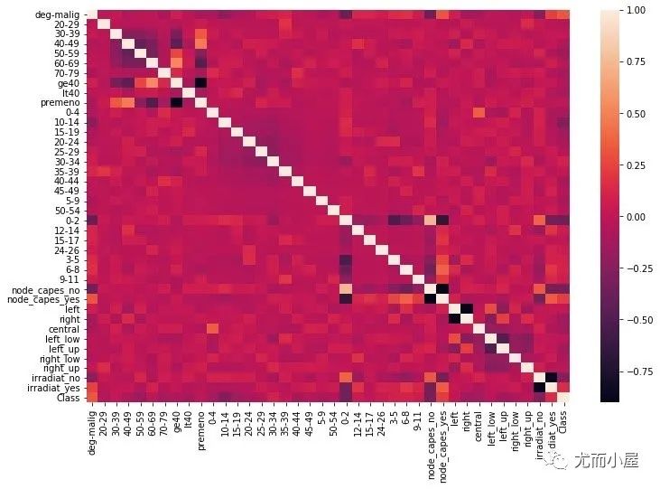
繪制相關(guān)性熱力圖:
fig?=?plt.figure(figsize=(12,8))
sns.heatmap(corr)

plt.show()
數(shù)據(jù)集劃分
In [38]:
X?=?df_smoted.iloc[:,:-1]
y?=?df_smoted.iloc[:,-1]

from?sklearn.model_selection?import?train_test_split

X_train,X_test,y_train,y_test?=?train_test_split(X,y,
?????????????????????????????????????????????????test_size=0.20,
?????????????????????????????????????????????????random_state=123)
決策樹
In [39]:
dt?=?DecisionTreeClassifier(max_depth=5)
dt.fit(X_train,?y_train)
Out[39]:
DecisionTreeClassifier(max_depth=5)
In [40]:
#?預(yù)測(cè)
y_prob?=?dt.predict_proba(X_test)[:,1]

#?預(yù)測(cè)的概率轉(zhuǎn)成0-1分類
y_pred?=?np.where(y_prob?>?0.5,?1,?0)
dt.score(X_test,?y_pred)
Out[40]:
1.0
In [41]:
#?混淆矩陣

confusion_matrix(y_test,?y_pred)
Out[41]:
array([[29,??8],
???????[19,?23]])
In [42]:
#?分類得分報(bào)告
print(classification_report(y_test,?y_pred))
??????????????precision????recall??f1-score???support

???????????0???????0.60??????0.78??????0.68????????37
???????????1???????0.74??????0.55??????0.63????????42

????accuracy???????????????????????????0.66????????79
???macro?avg???????0.67??????0.67??????0.66????????79
weighted?avg???????0.68??????0.66??????0.65????????79
In [43]:
#?roc
metrics.roc_auc_score(y_test,?y_pred)
Out[43]:
0.6657014157014157
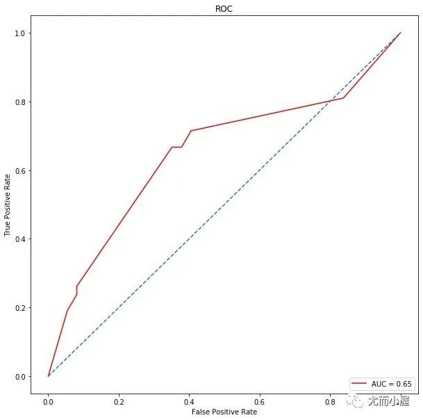
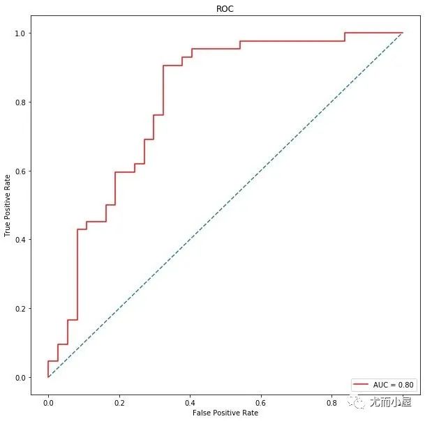
In [44]:
#?roc曲線

from?sklearn.metrics?import?roc_curve,?auc
false_positive_rate,?true_positive_rate,?thresholds?=?roc_curve(y_test,?y_prob)
roc_auc?=?auc(false_positive_rate,?true_positive_rate)

import?matplotlib.pyplot?as?plt
plt.figure(figsize=(10,10))??#?畫布
plt.title('ROC')??#?標(biāo)題

plt.plot(false_positive_rate,??#?繪圖
?????????true_positive_rate,
?????????color='red',
?????????label?=?'AUC?=?%0.2f'?%?roc_auc)

plt.legend(loc?=?'lower?right')?#??圖例位置
plt.plot([0,?1],?[0,?1],linestyle='--')??#?正比例直線

plt.axis('tight')
plt.xlabel('False?Positive?Rate')
plt.ylabel('True?Positive?Rate')
plt.show()
隨機(jī)森林
In [45]:
rf?=?RandomForestClassifier(max_depth=5)
rf.fit(X_train,?y_train)
梯度提升樹
In [50]:
from?sklearn.ensemble?import?GradientBoostingClassifier
In [51]:
gbc?=?GradientBoostingClassifier(loss='deviance',?
?????????????????????????????????learning_rate=0.1,?
?????????????????????????????????n_estimators=5,?
?????????????????????????????????subsample=1,
?????????????????????????????????min_samples_split=2,?
?????????????????????????????????min_samples_leaf=1,?
?????????????????????????????????max_depth=3)

gbc.fit(X_train,?y_train)
Out[51]:
GradientBoostingClassifier(n_estimators=5,?subsample=1)
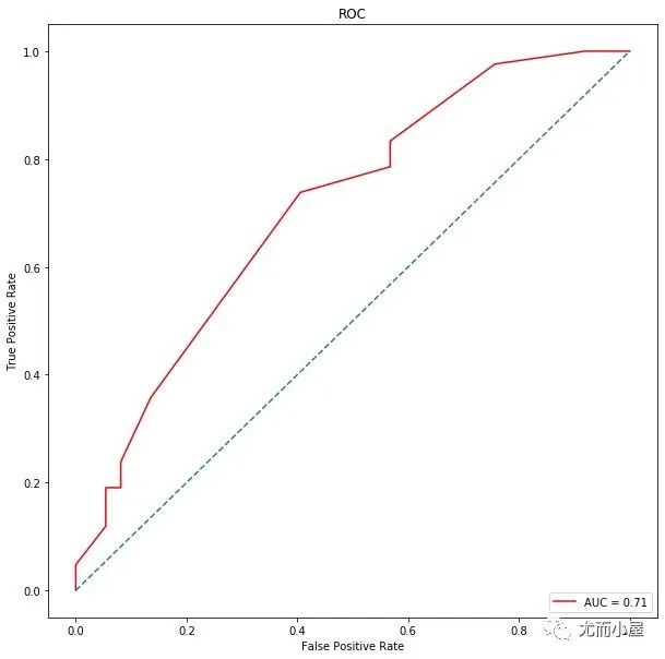
In [55]:
#?roc曲線

from?sklearn.metrics?import?roc_curve,?auc
false_positive_rate,?true_positive_rate,?thresholds?=?roc_curve(y_test,?y_prob)
roc_auc?=?auc(false_positive_rate,?true_positive_rate)

import?matplotlib.pyplot?as?plt
plt.figure(figsize=(10,10))??#?畫布
plt.title('ROC')??#?標(biāo)題

plt.plot(false_positive_rate,??#?繪圖
?????????true_positive_rate,
?????????color='red',
?????????label?=?'AUC?=?%0.2f'?%?roc_auc)

plt.legend(loc?=?'lower?right')?#??圖例位置
plt.plot([0,?1],?[0,?1],linestyle='--')??#?正比例直線

plt.axis('tight')
plt.xlabel('False?Positive?Rate')
plt.ylabel('True?Positive?Rate')
plt.show()
PCA降維
降維過(guò)程
In [56]:
from?sklearn.decomposition?import?PCA
pca?=?PCA(n_components=17)
pca.fit(X)

#返回所保留的17個(gè)成分各自的方差百分比
print(pca.explained_variance_ratio_)
[0.17513053?0.12941834?0.11453698?0.07323991?0.05889187?0.05690304
?0.04869476?0.0393374??0.03703477?0.03240863?0.03062932?0.02574137
?0.01887462?0.0180381??0.01606983?0.01453912?0.01318003]
In [57]:
sum(pca.explained_variance_ratio_)
Out[57]:
0.9026686181152915
降維后數(shù)據(jù)
In [58]:
X_NEW?=?pca.transform(X)
X_NEW
Out[58]:
array([[?1.70510215e-01,??5.39929099e-01,?-1.04314303e+00,?...,
????????-2.26541223e-01,?-6.39332871e-02,?-8.97923150e-02],
???????[-9.01105403e-01,??8.01693088e-01,??5.92260258e-01,?...,
?????????9.66299251e-02,??1.40755806e-03,?-2.74626972e-01],
???????[-6.05200264e-01,??6.08455330e-01,?-1.00524376e+00,?...,
?????????4.11416630e-02,??4.15705282e-02,?-8.46941345e-02],
???????...,
???????[?1.40652211e-02,??5.35906106e-01,??5.64150123e-02,?...,
?????????1.70834934e-01,??7.11616391e-02,?-1.72250445e-01],
???????[-4.41363597e-01,??9.11950641e-01,?-4.22184256e-01,?...,
????????-4.13385344e-02,?-7.64405982e-02,??1.04686148e-01],
???????[?1.98533663e+00,?-4.74547396e-01,?-1.52557494e-01,?...,
?????????2.72194184e-02,??5.71553613e-02,??1.78074886e-01]])
In [59]:
X_NEW.shape
Out[59]:
(392,?17)
重新劃分?jǐn)?shù)據(jù)
In [60]:
X_train,X_test,y_train,y_test?=?train_test_split(X_NEW,y,test_size=0.20,random_state=123)
再用隨機(jī)森林
In [61]:
rf?=?RandomForestClassifier(max_depth=5)
rf.fit(X_train,?y_train)
Out[61]:
RandomForestClassifier(max_depth=5)
In [62]:
#?預(yù)測(cè)
y_prob?=?rf.predict_proba(X_test)[:,1]

#?預(yù)測(cè)的概率轉(zhuǎn)成0-1分類
y_pred?=?np.where(y_prob?>?0.5,?1,?0)
rf.score(X_test,?y_pred)
Out[62]:
1.0
In [63]:
#?混淆矩陣

confusion_matrix(y_test,?y_pred)
Out[63]:
array([[26,?11],
???????[13,?29]])
In [64]:
#?roc
metrics.roc_auc_score(y_test,?y_pred)
Out[64]:
0.6965894465894465
In [65]:
#?roc曲線

from?sklearn.metrics?import?roc_curve,?auc
false_positive_rate,?true_positive_rate,?thresholds?=?roc_curve(y_test,?y_prob)
roc_auc?=?auc(false_positive_rate,?true_positive_rate)

import?matplotlib.pyplot?as?plt
plt.figure(figsize=(10,10))??
plt.title('ROC')??

plt.plot(false_positive_rate,??
?????????true_positive_rate,
?????????color='red',
?????????label?=?'AUC?=?%0.2f'?%?roc_auc)

plt.legend(loc?=?'lower?right')?
plt.plot([0,?1],?[0,?1],linestyle='--')??

plt.axis('tight')
plt.xlabel('False?Positive?Rate')
plt.ylabel('True?Positive?Rate')
plt.show()
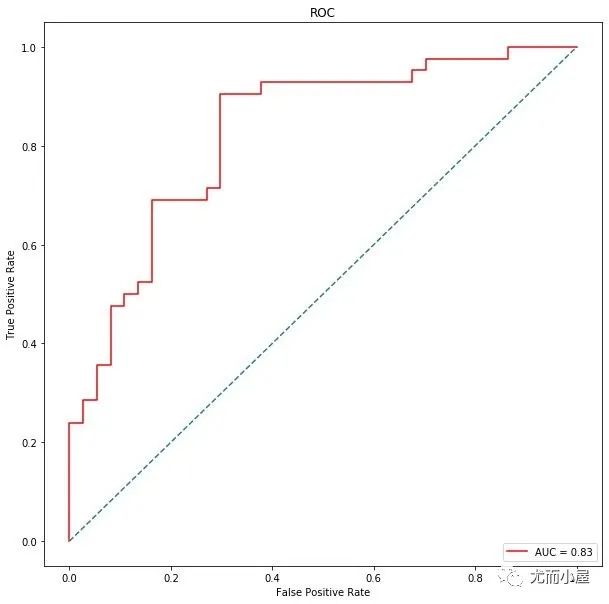
總結(jié)
從數(shù)據(jù)預(yù)處理和特征工程出發(fā),建立不同的樹模型表現(xiàn)來(lái)看,隨機(jī)森林表現(xiàn)的最好,AUC值高達(dá)0.81,在經(jīng)過(guò)對(duì)特征簡(jiǎn)單的降維之后,我們選擇前17個(gè)特征,它們的重要性超過(guò)90%,再次建模,此時(shí)AUC值達(dá)到0.83。
往期精彩回顧
適合初學(xué)者入門人工智能的路線及資料下載 (圖文+視頻)機(jī)器學(xué)習(xí)入門系列下載 中國(guó)大學(xué)慕課《機(jī)器學(xué)習(xí)》(黃海廣主講) 機(jī)器學(xué)習(xí)及深度學(xué)習(xí)筆記等資料打印 《統(tǒng)計(jì)學(xué)習(xí)方法》的代碼復(fù)現(xiàn)專輯 機(jī)器學(xué)習(xí)交流qq群955171419,加入微信群請(qǐng)掃碼