
Seaborn 繪制 21 種超實(shí)用精美圖表
大家好,我是云朵君!
導(dǎo)讀:?做過可視化的小伙伴們都會(huì)經(jīng)常聽到seaborn可視化,也有很多大佬平時(shí)使用的較多的可視化庫,今天我們就來盤下他,看看他有多實(shí)在。這里為了方便大家后面去練習(xí),所有展示數(shù)據(jù)均可從官網(wǎng)下載。

Python可視化庫Seaborn基于matplotlib,并提供了繪制吸引人的統(tǒng)計(jì)圖形的高級(jí)接口。
Seaborn就是讓困難的東西更加簡(jiǎn)單。它是針對(duì)統(tǒng)計(jì)繪圖的,一般來說,能滿足數(shù)據(jù)分析90%的繪圖需求。Seaborn其實(shí)是在matplotlib的基礎(chǔ)上進(jìn)行了更高級(jí)的API封裝,從而使得作圖更加容易,在大多數(shù)情況下使用seaborn就能做出很具有吸引力的圖,應(yīng)該把Seaborn視為matplotlib的補(bǔ)充,而不是替代物。同時(shí)它能高度兼容numpy與pandas數(shù)據(jù)結(jié)構(gòu)以及scipy與statsmodels等統(tǒng)計(jì)模式。
seaborn一共有5個(gè)大類21種圖,分別是:
Relational plots 關(guān)系類圖表
relplot 關(guān)系類圖表的接口,其實(shí)是下面兩種圖的集成,通過指定kind參數(shù)可以畫出下面的兩種圖 scatterplot 散點(diǎn)圖 lineplot 折線圖
Categorical plots 分類圖表 catplot 分類圖表的接口,其實(shí)是下面八種圖表的集成,,通過指定kind參數(shù)可以畫出下面的八種圖
stripplot 分類散點(diǎn)圖 swarmplot 能夠顯示分布密度的分類散點(diǎn)圖 boxplot 箱圖 violinplot 小提琴圖 boxenplot 增強(qiáng)箱圖 pointplot 點(diǎn)圖 barplot 條形圖 countplot 計(jì)數(shù)圖
Distribution plot 分布圖
jointplot 雙變量關(guān)系圖 pairplot 變量關(guān)系組圖 distplot 直方圖,質(zhì)量估計(jì)圖 kdeplot 核函數(shù)密度估計(jì)圖 rugplot 將數(shù)組中的數(shù)據(jù)點(diǎn)繪制為軸上的數(shù)據(jù)
Regression plots 回歸圖
lmplot 回歸模型圖 regplot 線性回歸圖 residplot 線性回歸殘差圖
Matrix plots 矩陣圖
heatmap 熱力圖 clustermap 聚集圖
導(dǎo)入模塊
使用以下別名來導(dǎo)入庫:
import?matplotlib.pyplot?as?plt
import?seaborn?as?sns
使用Seaborn創(chuàng)建圖形的基本步驟是:
準(zhǔn)備一些數(shù)據(jù) 控制圖美觀 Seaborn繪圖 進(jìn)一步定制你的圖形 展示圖形
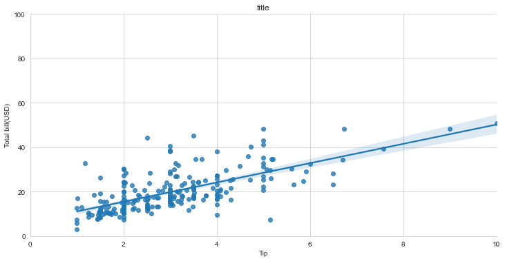
import?matplotlib.pyplot?as?plt?
import?seaborn?as?sns
tips?=?sns.load_dataset("tips")????#?Step?1
sns.set_style("whitegrid")?????????#?Step?2?
g?=?sns.lmplot(x="tip",????????????#?Step?3
???????????????y="total_bill",
???????????????data=tips,
???????????????aspect=2)????????????
g?=?(g.set_axis_labels("Tip","Total?bill(USD)")?\
????.set(xlim=(0,10),ylim=(0,100)))?????????????????????????????????????????????????????????????????????????????????????
plt.title("title")?????????????????#?Step?4
plt.show(g)?
若要在NoteBook中展示圖形,可使用魔法函數(shù):
%matplotlib?inline
數(shù)據(jù)準(zhǔn)備
import?pandas?as?pd
import?numpy?as?np
uniform_data?=?np.random.rand(10,?12)
data?=?pd.DataFrame({'x':np.arange(1,101),
?????????????????????'y':np.random.normal(0,4,100)})
Seaborn還提供內(nèi)置數(shù)據(jù)集
#?直接加載,到網(wǎng)上拉取數(shù)據(jù)
titanic?=?sns.load_dataset("titanic")
iris?=?sns.load_dataset("iris")
#?如果下載較慢,或加載失敗,可以下載到本地,然后加載本地路徑
titanic?=?sns.load_dataset('titanic',data_home='seaborn-data',cache=True)
iris?=?sns.load_dataset("iris",data_home='seaborn-data',cache=True)
下載地址:https://github.com/mwaskom/seaborn-data
圖片美觀
創(chuàng)建畫布
#?創(chuàng)建畫布和一個(gè)子圖
f,?ax?=?plt.subplots(figsize=(5,6))
Seaborn 樣式
sns.set()???#(重新)設(shè)置seaborn的默認(rèn)值
sns.set_style("whitegrid")????#設(shè)置matplotlib參數(shù)
sns.set_style("ticks",????????#設(shè)置matplotlib參數(shù)
?????????????{"xtick.major.size":?8,?
??????????????"ytick.major.size":?8})
sns.axes_style("whitegrid")???#返回一個(gè)由參數(shù)組成的字典,或使用with來臨時(shí)設(shè)置樣式
設(shè)置繪圖上下文參數(shù)
sns.set_context("talk")????????#?設(shè)置上下文為“talk”

sns.set_context("notebook",???#?設(shè)置上下文為"notebook",縮放字體元素和覆蓋參數(shù)映射
????????????????font_scale=1.5,?
????????????????rc={"lines.linewidth":2.5})
調(diào)色板
sns.set_palette("husl",3)?#?定義調(diào)色板
sns.color_palette("husl")?#?用with使用臨時(shí)設(shè)置調(diào)色板

flatui?=?["#9b59b6","#3498db","#95a5a6",
??????????"#e74c3c","#34495e","#2ecc71"]?
sns.set_palette(flatui)??#?自定義調(diào)色板
Axisgrid 對(duì)象設(shè)置
g.despine(left=True)??????#?隱藏左邊線?
g.set_ylabels("Survived")?#?設(shè)置y軸的標(biāo)簽
g.set_xticklabels(rotation=45)??????#?為x設(shè)置刻度標(biāo)簽
g.set_axis_labels("Survived","Sex")?#?設(shè)置軸標(biāo)簽
h.set(xlim=(0,5),?????????#?設(shè)置x軸和y軸的極限和刻度
??????ylim=(0,5),
??????xticks=[0,2.5,5],
??????yticks=[0,2.5,5])
plt設(shè)置
plt.title("A?Title")????#?添加圖標(biāo)題
plt.ylabel("Survived")??#?調(diào)整y軸標(biāo)簽
plt.xlabel("Sex")???????#?調(diào)整x軸的標(biāo)簽
plt.ylim(0,100)?????????#?調(diào)整y軸的上下限
plt.xlim(0,10)??????????#?調(diào)整x軸的限制
plt.setp(ax,yticks=[0,5])?#?調(diào)整繪圖屬性
plt.tight_layout()??????#?次要情節(jié)調(diào)整參數(shù)
展示或保存圖片
plt.show()
plt.savefig("foo.png")
plt.savefig("foo.png",???#?保存透明圖片
????????????transparent=True)

plt.cla()???#?清除軸
plt.clf()???#?清除整個(gè)圖片
plt.close()?#?關(guān)閉窗口
Seaborn繪圖
relplot
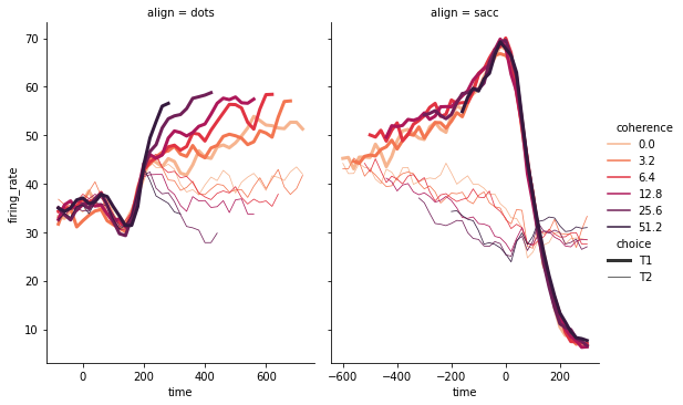
這是一個(gè)圖形級(jí)別的函數(shù),它用散點(diǎn)圖和線圖兩種常用的手段來表現(xiàn)統(tǒng)計(jì)關(guān)系。hue, col分類依據(jù),size將產(chǎn)生不同大小的元素的變量分組,aspect長(zhǎng)寬比,legend_full每組均有條目。
dots?=?sns.load_dataset('dots',
????????????data_home='seaborn-data',
????????????cache=True)
#?將調(diào)色板定義為一個(gè)列表,以指定精確的值
palette?=?sns.color_palette("rocket_r")

#?在兩個(gè)切面上畫線
sns.relplot(
????data=dots,
????x="time",?y="firing_rate",
????hue="coherence",?size="choice",?
????col="align",?kind="line",?
????size_order=["T1",?"T2"],?palette=palette,
????height=5,?aspect=.75,?
????facet_kws=dict(sharex=False),
)
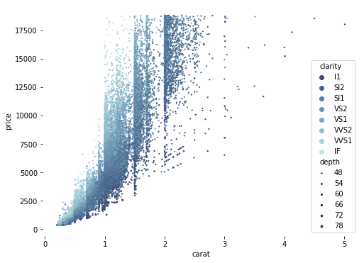
散點(diǎn)圖scatterplot
diamonds?=?sns.load_dataset('diamonds',data_home='seaborn-data',cache=True)

#?繪制散點(diǎn)圖,同時(shí)指定不同的點(diǎn)顏色和大小
f,?ax?=?plt.subplots(figsize=(8,?6))
sns.despine(f,?left=True,?bottom=True)
clarity_ranking?=?["I1",?"SI2",?"SI1",?"VS2",?"VS1",?"VVS2",?"VVS1",?"IF"]
sns.scatterplot(x="carat",?y="price",
????????????????hue="clarity",?size="depth",
????????????????palette="ch:r=-.2,d=.3_r",
????????????????hue_order=clarity_ranking,
????????????????sizes=(1,?8),?linewidth=0,
????????????????data=diamonds,?ax=ax)
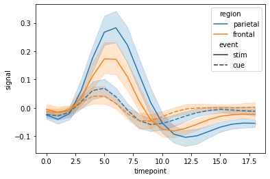
折線圖lineplot
seaborn里的lineplot函數(shù)所傳數(shù)據(jù)必須為一個(gè)pandas數(shù)組。
fmri?=?sns.load_dataset('fmri',data_home='seaborn-data',cache=True)
#?繪制不同事件和地區(qū)的響應(yīng)
sns.lineplot(x="timepoint",?y="signal",
?????????????hue="region",?style="event",
?????????????data=fmri)
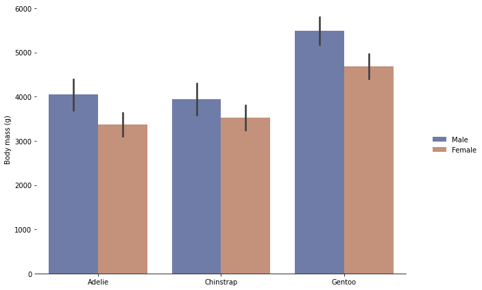
成組的柱狀圖catplot
分類圖表的接口,通過指定kind參數(shù)可以畫出下面的八種圖
stripplot 分類散點(diǎn)圖
swarmplot 能夠顯示分布密度的分類散點(diǎn)圖
boxplot 箱圖
violinplot 小提琴圖
boxenplot 增強(qiáng)箱圖
pointplot 點(diǎn)圖
barplot 條形圖
countplot 計(jì)數(shù)圖
penguins?=?sns.load_dataset('penguins',data_home='seaborn-data',cache=True)
#?按物種和性別畫一個(gè)嵌套的引線圖
g?=?sns.catplot(
????data=penguins,?kind="bar",
????x="species",?y="body_mass_g",?hue="sex",
????ci="sd",?palette="dark",?alpha=.6,?height=6)
g.despine(left=True)
g.set_axis_labels("",?"Body?mass?(g)")
g.legend.set_title("")
g.fig.set_size_inches(10,6)?#?設(shè)置畫布大小
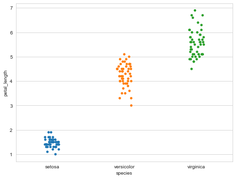
分類散點(diǎn)圖stripplot
sns.stripplot(x="species",
??????????????y="petal_length",
??????????????data=iris)
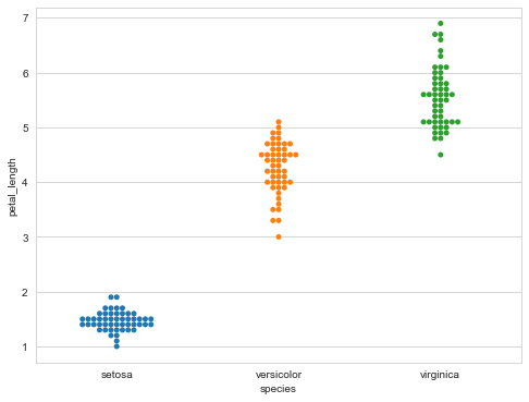
無重疊點(diǎn)的分類散點(diǎn)圖swarmplot
能夠顯示分布密度的分類散點(diǎn)圖。
sns.swarmplot(x="species",
??????????????y="petal_length",
??????????????data=iris)
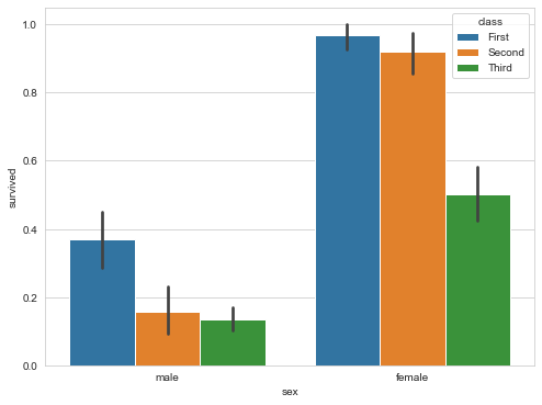
柱狀圖barplot
用散點(diǎn)符號(hào)顯示點(diǎn)估計(jì)和置信區(qū)間。
sns.barplot(x="sex",
????????????y="survived",
????????????hue="class",
????????????data=titanic)
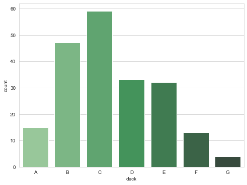
計(jì)數(shù)圖countplot
#?顯示觀測(cè)次數(shù)
sns.countplot(x="deck",
??????????????data=titanic,
??????????????palette="Greens_d")
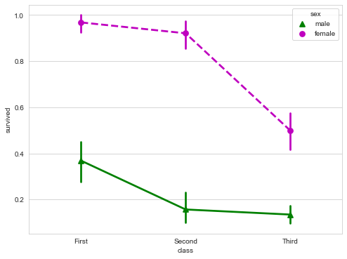
點(diǎn)圖pointplot
用矩形條顯示點(diǎn)估計(jì)和置信區(qū)間。
點(diǎn)圖代表散點(diǎn)圖位置的數(shù)值變量的中心趨勢(shì)估計(jì),并使用誤差線提供關(guān)于該估計(jì)的不確定性的一些指示。點(diǎn)圖可能比條形圖更有用于聚焦一個(gè)或多個(gè)分類變量的不同級(jí)別之間的比較。他們尤其善于表現(xiàn)交互作用:一個(gè)分類變量的層次之間的關(guān)系如何在第二個(gè)分類變量的層次之間變化。連接來自相同色調(diào)等級(jí)的每個(gè)點(diǎn)的線允許交互作用通過斜率的差異進(jìn)行判斷,這比對(duì)幾組點(diǎn)或條的高度比較容易。
sns.pointplot(x="class",
??????????????y="survived",
??????????????hue="sex",
??????????????data=titanic,
??????????????palette={"male":"g",?"female":"m"},
??????????????markers=["^","o"],
??????????????linestyles=["-","--"])
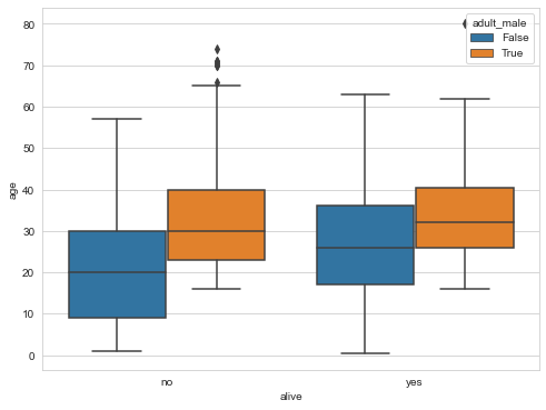
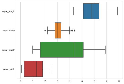
箱形圖boxplot
箱形圖(Box-plot)又稱為盒須圖、盒式圖或箱線圖,是一種用作顯示一組數(shù)據(jù)分散情況資料的統(tǒng)計(jì)圖。它能顯示出一組數(shù)據(jù)的最大值、最小值、中位數(shù)及上下四分位數(shù)。
sns.boxplot(x="alive",
????????????y="age",
????????????hue="adult_male",?#?hue分類依據(jù)
????????????data=titanic)
#?繪制寬表數(shù)據(jù)箱形圖
sns.boxplot(data=iris,orient="h")
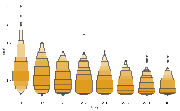
增強(qiáng)箱圖boxenplot
boxenplot是為更大的數(shù)據(jù)集繪制增強(qiáng)的箱型圖。這種風(fēng)格的繪圖最初被命名為“信值圖”,因?yàn)樗@示了大量被定義為“置信區(qū)間”的分位數(shù)。它類似于繪制分布的非參數(shù)表示的箱形圖,其中所有特征對(duì)應(yīng)于實(shí)際觀察的數(shù)值點(diǎn)。通過繪制更多分位數(shù),它提供了有關(guān)分布形狀的更多信息,特別是尾部數(shù)據(jù)的分布。
clarity_ranking?=?["I1",?"SI2",?"SI1",?"VS2",?"VS1",?"VVS2",?"VVS1",?"IF"]
f,?ax?=?plt.subplots(figsize=(10,?6))
sns.boxenplot(x="clarity",?y="carat",
??????????????color="orange",?order=clarity_ranking,
??????????????scale="linear",?data=diamonds,ax=ax)
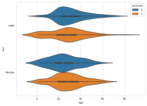
小提琴圖violinplot
violinplot與boxplot扮演類似的角色,它顯示了定量數(shù)據(jù)在一個(gè)(或多個(gè))分類變量的多個(gè)層次上的分布,這些分布可以進(jìn)行比較。不像箱形圖中所有繪圖組件都對(duì)應(yīng)于實(shí)際數(shù)據(jù)點(diǎn),小提琴繪圖以基礎(chǔ)分布的核密度估計(jì)為特征。
sns.violinplot(x="age",
???????????????y="sex",
???????????????hue="survived",
???????????????data=titanic)
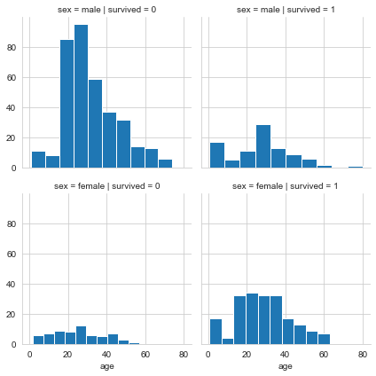
繪制條件關(guān)系的網(wǎng)格FacetGrid
FacetGrid是一個(gè)繪制多個(gè)圖表(以網(wǎng)格形式顯示)的接口。
g?=?sns.FacetGrid(titanic,
??????????????????col="survived",
??????????????????row="sex")
g?=?g.map(plt.hist,"age")
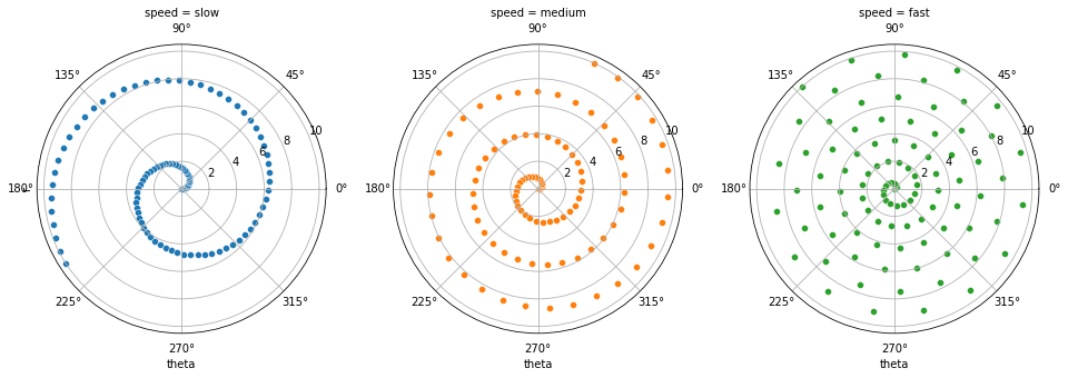
極坐標(biāo)網(wǎng)絡(luò)FacetGrid
#?生成一個(gè)例子徑向數(shù)據(jù)集
r?=?np.linspace(0,?10,?num=100)
df?=?pd.DataFrame({'r':?r,?'slow':?r,?'medium':?2?*?r,?'fast':?4?*?r})
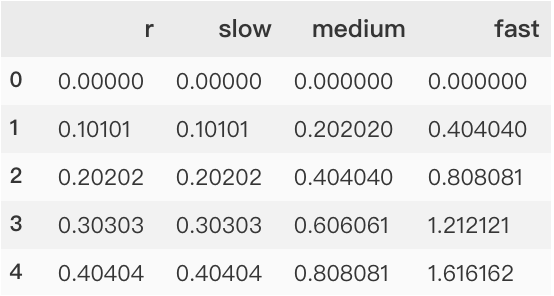
#?將dataframe轉(zhuǎn)換為長(zhǎng)格式或“整齊”格式
df?=?pd.melt(df,?id_vars=['r'],?var_name='speed',?value_name='theta')
#?用極投影建立一個(gè)坐標(biāo)軸網(wǎng)格
g?=?sns.FacetGrid(df,?col="speed",?hue="speed",
??????????????????subplot_kws=dict(projection='polar'),?height=4.5,
??????????????????sharex=False,?sharey=False,?despine=False)
#?在網(wǎng)格的每個(gè)軸上畫一個(gè)散點(diǎn)圖
g.map(sns.scatterplot,?"theta",?"r")
將dataframe轉(zhuǎn)換為長(zhǎng)格式或“整齊”格式過程
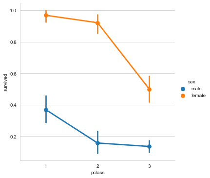
分類圖factorplot
#?在Facetgrid上繪制一個(gè)分類圖
sns.factorplot(x="pclass",
???????????????y="survived",
???????????????hue="sex",
???????????????data=titanic)
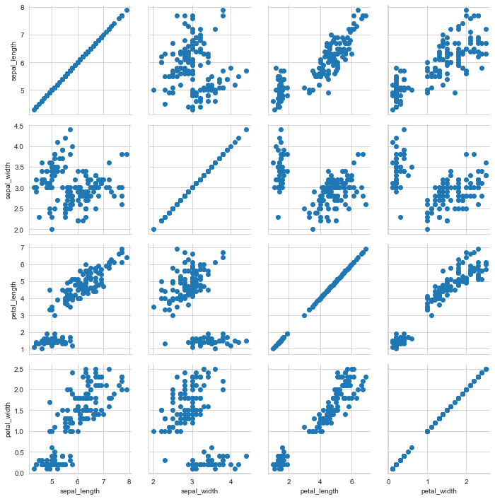
成對(duì)關(guān)系網(wǎng)格圖PairGrid
h?=?sns.PairGrid(iris)????#?繪制成對(duì)關(guān)系的Subplot網(wǎng)格圖
h?=?h.map(plt.scatter)
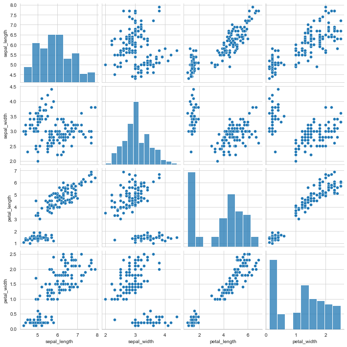
雙變量分布pairplot
變量關(guān)系組圖。
sns.pairplot(iris)????????#?繪制雙變量分布
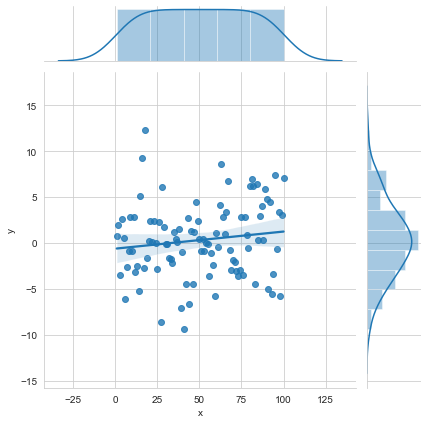
雙變量圖的網(wǎng)格與邊緣單變量圖JointGrid
i?=?sns.JointGrid(x="x",??#?雙變量圖的網(wǎng)格與邊緣單變量圖
??????????????????y="y",
??????????????????data=data)
i?=?i.plot(sns.regplot,
???????????sns.distplot)
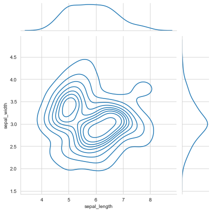
二維分布jointplot
用于兩個(gè)變量的畫圖,將兩個(gè)變量的聯(lián)合分布形態(tài)可視化出來往往會(huì)很有用。在seaborn中,最簡(jiǎn)單的實(shí)現(xiàn)方式是使用jointplot函數(shù),它會(huì)生成多個(gè)面板,不僅展示了兩個(gè)變量之間的關(guān)系,也在兩個(gè)坐標(biāo)軸上分別展示了每個(gè)變量的分布。
sns.jointplot("sepal_length",??#?繪制二維分布
??????????????"sepal_width",
??????????????data=iris,
??????????????kind='kde'?#?kind=?"hex"就是兩個(gè)坐標(biāo)軸上顯示直方圖
?????????????)
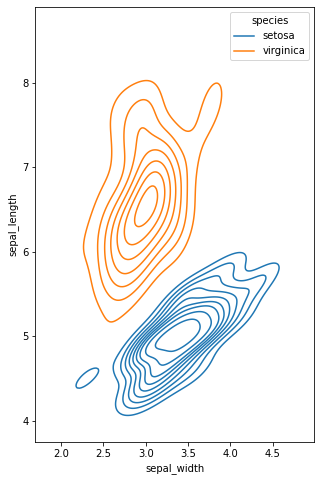
多元雙變量核密度估計(jì)kdeplot
核密度估計(jì)(kernel density estimation)是在概率論中用來估計(jì)未知的密度函數(shù),屬于非參數(shù)檢驗(yàn)方法之一。通過核密度估計(jì)圖可以比較直觀的看出數(shù)據(jù)樣本本身的分布特征。
f,?ax?=?plt.subplots(figsize=(8,?8))
ax.set_aspect("equal")

#?繪制等高線圖來表示每一個(gè)二元密度
sns.kdeplot(
????data=iris.query("species?!=?'versicolor'"),
????x="sepal_width",
????y="sepal_length",
????hue="species",
????thresh=.1,)
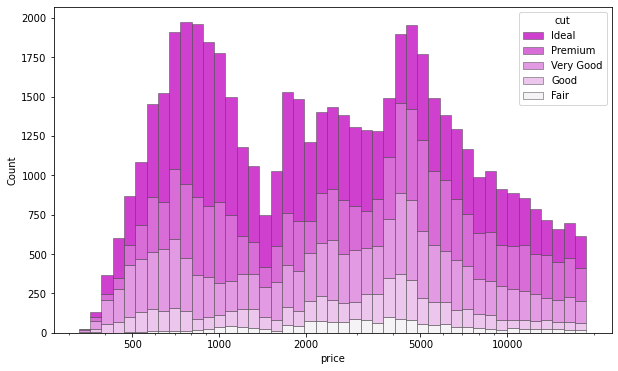
多變量直方圖histplot
繪制單變量或雙變量直方圖以顯示數(shù)據(jù)集的分布。
直方圖是一種典型的可視化工具,它通過計(jì)算離散箱中的觀察值數(shù)量來表示一個(gè)或多個(gè)變量的分布。該函數(shù)可以對(duì)每個(gè)箱子內(nèi)計(jì)算的統(tǒng)計(jì)數(shù)據(jù)進(jìn)行歸一化,以估計(jì)頻率、密度或概率質(zhì)量,并且可以添加使用核密度估計(jì)獲得的平滑曲線,類似于?kdeplot()。
f,?ax?=?plt.subplots(figsize=(10,?6))
sns.histplot(
????diamonds,
????x="price",?hue="cut",
????multiple="stack",
????palette="light:m_r",
????edgecolor=".3",
????linewidth=.5,
????log_scale=True,
)
ax.xaxis.set_major_formatter(mpl.ticker.ScalarFormatter())
ax.set_xticks([500,?1000,?2000,?5000,?10000])
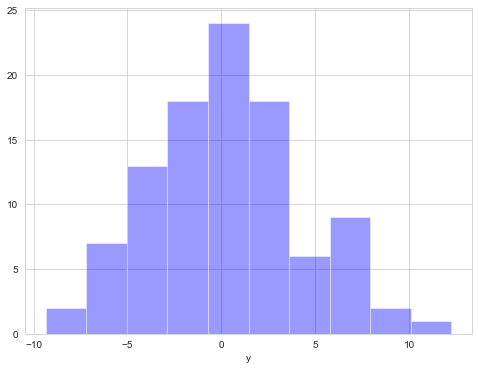
單變量分布圖distplot
在seaborn中想要對(duì)單變量分布進(jìn)行快速了解最方便的就是使用distplot函數(shù),默認(rèn)情況下它將繪制一個(gè)直方圖,并且可以同時(shí)畫出核密度估計(jì)(KDE)。
plot?=?sns.distplot(data.y,
????????????????????kde=False,
????????????????????color='b')
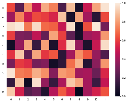
矩陣圖heatmap
利用熱力圖可以看數(shù)據(jù)表里多個(gè)特征兩兩的相似度。
sns.heatmap(uniform_data,vmin=0,vmax=1)
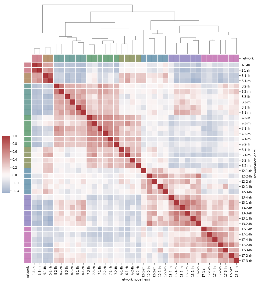
分層聚集的熱圖clustermap
#?Load?the?brain?networks?example?dataset
df?=?sns.load_dataset("brain_networks",?header=[0,?1,?2],?index_col=0,data_home='seaborn-data',cache=True)

#?選擇networks網(wǎng)絡(luò)的一個(gè)子集
used_networks?=?[1,?5,?6,?7,?8,?12,?13,?17]
used_columns?=?(df.columns.get_level_values("network")
??????????????????????????.astype(int)
??????????????????????????.isin(used_networks))
df?=?df.loc[:,?used_columns]

#?創(chuàng)建一個(gè)分類調(diào)色板來識(shí)別網(wǎng)絡(luò)networks
network_pal?=?sns.husl_palette(8,?s=.45)
network_lut?=?dict(zip(map(str,?used_networks),?network_pal))

#?將調(diào)色板轉(zhuǎn)換為將繪制在矩陣邊的矢量
networks?=?df.columns.get_level_values("network")
network_colors?=?pd.Series(networks,?index=df.columns).map(network_lut)

#?繪制完整的圖
g?=?sns.clustermap(df.corr(),?center=0,?cmap="vlag",
???????????????????row_colors=network_colors,?col_colors=network_colors,
???????????????????dendrogram_ratio=(.1,?.2),
???????????????????cbar_pos=(.02,?.32,?.03,?.2),
???????????????????linewidths=.75,?figsize=(12,?13))

g.ax_row_dendrogram.remove()
推薦閱讀
牛逼!Python常用數(shù)據(jù)類型的基本操作(長(zhǎng)文系列第①篇)
牛逼!Python的判斷、循環(huán)和各種表達(dá)式(長(zhǎng)文系列第②篇)
推薦閱讀
牛逼!Python常用數(shù)據(jù)類型的基本操作(長(zhǎng)文系列第①篇)
牛逼!Python的判斷、循環(huán)和各種表達(dá)式(長(zhǎng)文系列第②篇)