
項(xiàng)目實(shí)踐 | 基于YOLO-V5實(shí)現(xiàn)行人社交距離風(fēng)險(xiǎn)提示(文末獲取完整源...
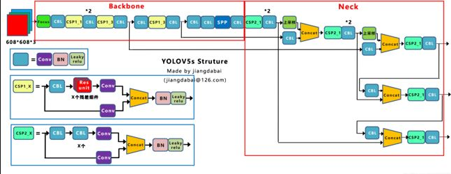
由于YOLO V5的作者現(xiàn)在并沒有發(fā)表論文,因此只能從代碼的角度理解它的工作。YOLO V5的網(wǎng)絡(luò)結(jié)構(gòu)圖如下:
1、與YOLO V4的區(qū)別
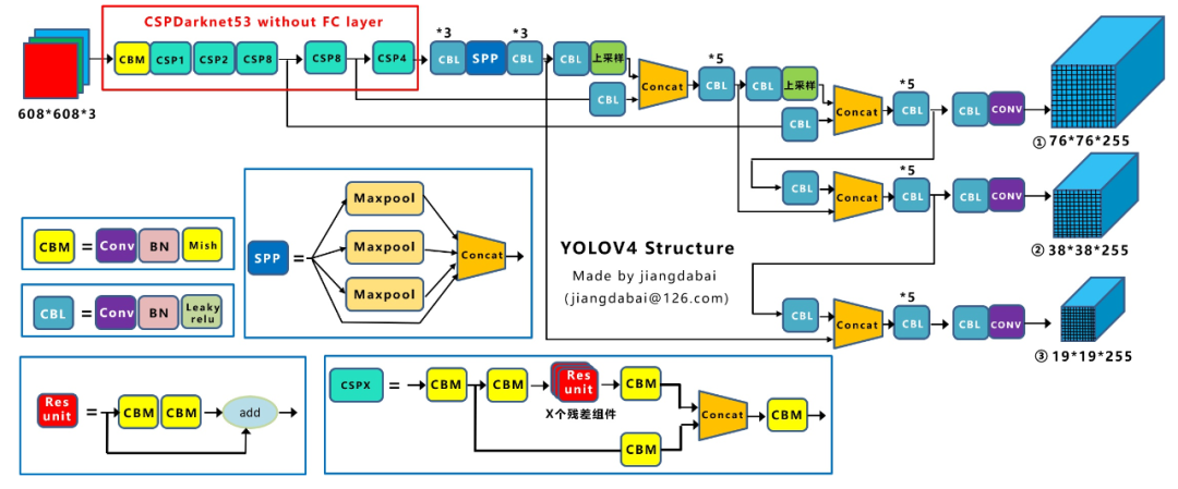
Yolov4在Yolov3的基礎(chǔ)上進(jìn)行了很多的創(chuàng)新。比如輸入端采用mosaic數(shù)據(jù)增強(qiáng),Backbone上采用了CSPDarknet53、Mish激活函數(shù)、Dropblock等方式,Neck中采用了SPP、FPN+PAN的結(jié)構(gòu),輸出端則采用CIOU_Loss、DIOU_nms操作。因此Yolov4對(duì)Yolov3的各個(gè)部分都進(jìn)行了很多的整合創(chuàng)新。這里給出YOLO V4的網(wǎng)絡(luò)結(jié)構(gòu)圖:
Yolov5的結(jié)構(gòu)其實(shí)和Yolov4的結(jié)構(gòu)還是有一定的相似之處的,但也有一些不同,這里還是按照從整體到細(xì)節(jié)的方式,對(duì)每個(gè)板塊進(jìn)行講解。這里給出YOLO V4的網(wǎng)絡(luò)結(jié)構(gòu)圖:
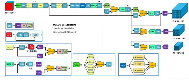
通過Yolov5的網(wǎng)絡(luò)結(jié)構(gòu)圖可以看到,依舊是把模型分為4個(gè)部分,分別是:輸入端、Backbone、Neck、Prediction。
1.1、輸入端的區(qū)別
1 Mosaic數(shù)據(jù)增強(qiáng)
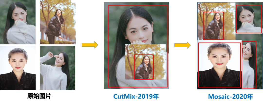
Mosaic是參考CutMix數(shù)據(jù)增強(qiáng)的方式,但CutMix只使用了兩張圖片進(jìn)行拼接,而Mosaic數(shù)據(jù)增強(qiáng)則采用了4張圖片,隨機(jī)縮放、隨機(jī)裁剪、隨機(jī)排布的方式進(jìn)行拼接。
主要有幾個(gè)優(yōu)點(diǎn):
1、豐富數(shù)據(jù)集:隨機(jī)使用4張圖片,隨機(jī)縮放,再隨機(jī)分布進(jìn)行拼接,大大豐富了檢測(cè)數(shù)據(jù)集,特別是隨機(jī)縮放增加了很多小目標(biāo),讓網(wǎng)絡(luò)的魯棒性更好。
2、減少GPU:可能會(huì)有人說,隨機(jī)縮放,普通的數(shù)據(jù)增強(qiáng)也可以做,但作者考慮到很多人可能只有一個(gè)GPU,因此Mosaic增強(qiáng)訓(xùn)練時(shí),可以直接計(jì)算4張圖片的數(shù)據(jù),使得Mini-batch大小并不需要很大,一個(gè)GPU就可以達(dá)到比較好的效果。
2 自適應(yīng)錨框計(jì)算
在Yolov3、Yolov4中,訓(xùn)練不同的數(shù)據(jù)集時(shí),計(jì)算初始錨框的值是通過單獨(dú)的程序運(yùn)行的。但Yolov5中將此功能嵌入到代碼中,每次訓(xùn)練時(shí),自適應(yīng)的計(jì)算不同訓(xùn)練集中的最佳錨框值。
比如Yolov5在Coco數(shù)據(jù)集上初始設(shè)定的錨框:
3 自適應(yīng)圖片縮放
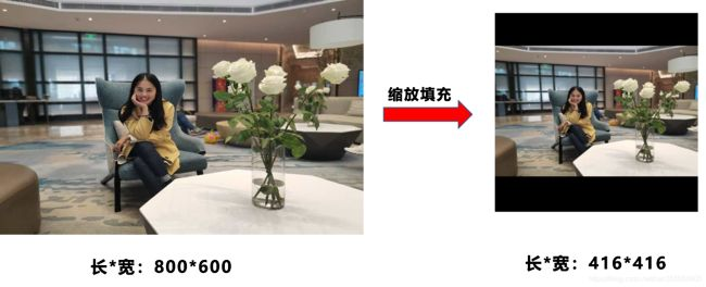
在常用的目標(biāo)檢測(cè)算法中,不同的圖片長(zhǎng)寬都不相同,因此常用的方式是將原始圖片統(tǒng)一縮放到一個(gè)標(biāo)準(zhǔn)尺寸,再送入檢測(cè)網(wǎng)絡(luò)中。比如Yolo算法中常用416×416,608×608等尺寸,比如對(duì)下面800×600的圖像進(jìn)行變換。
但Yolov5代碼中對(duì)此進(jìn)行了改進(jìn),也是Yolov5推理速度能夠很快的一個(gè)不錯(cuò)的trick。作者認(rèn)為,在項(xiàng)目實(shí)際使用時(shí),很多圖片的長(zhǎng)寬比不同。因此縮放填充后,兩端的黑邊大小都不同,而如果填充的比較多,則存在信息冗余,影響推理速度。
具體操作的步驟:
1 計(jì)算縮放比例
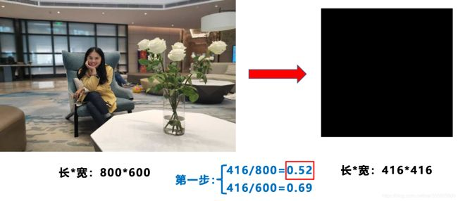 原始縮放尺寸是416×416,都除以原始圖像的尺寸后,可以得到0.52,和0.69兩個(gè)縮放系數(shù),選擇小的縮放系數(shù)0.52。
2 計(jì)算縮放后的尺寸
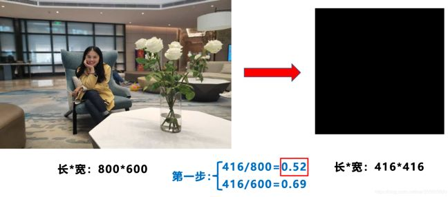
原始圖片的長(zhǎng)寬都乘以最小的縮放系數(shù)0.52,寬變成了416,而高變成了312。
3 計(jì)算黑邊填充數(shù)值
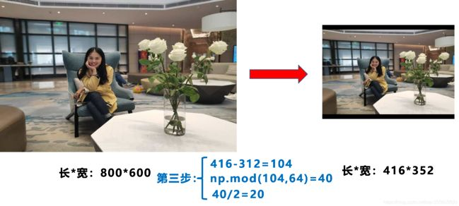
將416-312=104,得到原本需要填充的高度。再采用numpy中np.mod取余數(shù)的方式,得到40個(gè)像素,再除以2,即得到圖片高度兩端需要填充的數(shù)值。
1.2、Backbone的區(qū)別
1 Focus結(jié)構(gòu)
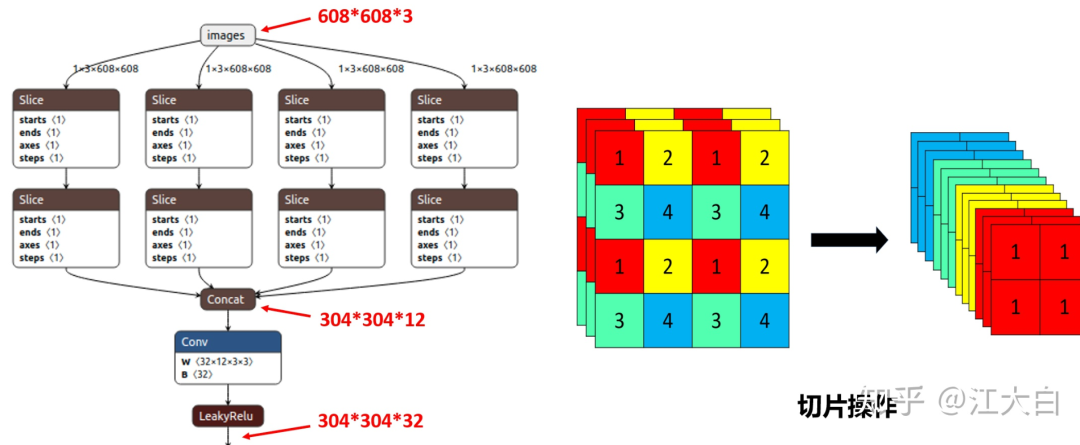
Focus結(jié)構(gòu),在Yolov3&Yolov4中并沒有這個(gè)結(jié)構(gòu),其中比較關(guān)鍵是切片操作。比如右圖的切片示意圖,4×4×3的圖像切片后變成3×3×12的特征圖。以Yolov5s的結(jié)構(gòu)為例,原始608×608×3的圖像輸入Focus結(jié)構(gòu),采用切片操作,先變成304×304×12的特征圖,再經(jīng)過一次32個(gè)卷積核的卷積操作,最終變成304×304×32的特征圖。
需要注意的是:Yolov5s的Focus結(jié)構(gòu)最后使用了32個(gè)卷積核,而其他三種結(jié)構(gòu),使用的數(shù)量有所增加,先注意下,后面會(huì)講解到四種結(jié)構(gòu)的不同點(diǎn)。
class Focus(nn.Module):
    # Focus wh information into c-space
    def __init__(self, c1, c2, k=1):
        super(Focus, self).__init__()
        self.conv = Conv(c1 * 4, c2, k, 1)

    def forward(self, x):  # x(b,c,w,h) -> y(b,4c,w/2,h/2)
        return self.conv(torch.cat([x[..., ::2, ::2], x[..., 1::2, ::2], x[..., ::2, 1::2], x[..., 1::2, 1::2]], 1))
2 CSP結(jié)構(gòu)
Yolov5與Yolov4不同點(diǎn)在于,Yolov4中只有主干網(wǎng)絡(luò)使用了CSP結(jié)構(gòu),而Yolov5中設(shè)計(jì)了兩種CSP結(jié)構(gòu),以Yolov5s網(wǎng)絡(luò)為例,以CSP1_X結(jié)構(gòu)應(yīng)用于Backbone主干網(wǎng)絡(luò),另一種CSP2_X結(jié)構(gòu)則應(yīng)用于Neck中。
class Conv(nn.Module):
    # Standard convolution
    def __init__(self, c1, c2, k=1, s=1, g=1, act=True):  # ch_in, ch_out, kernel, stride, groups
        super(Conv, self).__init__()
        self.conv = nn.Conv2d(c1, c2, k, s, k // 2, groups=g, bias=False)
        self.bn = nn.BatchNorm2d(c2)
        self.act = nn.LeakyReLU(0.1, inplace=True) if act else nn.Identity()

    def forward(self, x):
        return self.act(self.bn(self.conv(x)))

    def fuseforward(self, x):
        return self.act(self.conv(x))


class Bottleneck(nn.Module):
    # Standard bottleneck
    def __init__(self, c1, c2, shortcut=True, g=1, e=0.5):  # ch_in, ch_out, shortcut, groups, expansion
        super(Bottleneck, self).__init__()
        c_ = int(c2 * e)  # hidden channels
        self.cv1 = Conv(c1, c_, 1, 1)
        self.cv2 = Conv(c_, c2, 3, 1, g=g)
        self.add = shortcut and c1 == c2

    def forward(self, x):
        return x + self.cv2(self.cv1(x)) if self.add else self.cv2(self.cv1(x))


class BottleneckCSP(nn.Module):
    # CSP Bottleneck https://github.com/WongKinYiu/CrossStagePartialNetworks
    def __init__(self, c1, c2, n=1, shortcut=True, g=1, e=0.5):  # ch_in, ch_out, number, shortcut, groups, expansion
        super(BottleneckCSP, self).__init__()
        c_ = int(c2 * e)  # hidden channels
        self.cv1 = Conv(c1, c_, 1, 1)
        self.cv2 = nn.Conv2d(c1, c_, 1, 1, bias=False)
        self.cv3 = nn.Conv2d(c_, c_, 1, 1, bias=False)
        self.cv4 = Conv(c2, c2, 1, 1)
        self.bn = nn.BatchNorm2d(2 * c_)  # applied to cat(cv2, cv3)
        self.act = nn.LeakyReLU(0.1, inplace=True)
        self.m = nn.Sequential(*[Bottleneck(c_, c_, shortcut, g, e=1.0) for _ in range(n)])

    def forward(self, x):
        y1 = self.cv3(self.m(self.cv1(x)))
        y2 = self.cv2(x)
        return self.cv4(self.act(self.bn(torch.cat((y1, y2), dim=1))))
1.3、Neck的區(qū)別
Yolov5現(xiàn)在的Neck和Yolov4中一樣,都采用FPN+PAN的結(jié)構(gòu),但在Yolov5剛出來時(shí),只使用了FPN結(jié)構(gòu),后面才增加了PAN結(jié)構(gòu),此外網(wǎng)絡(luò)中其他部分也進(jìn)行了調(diào)整。
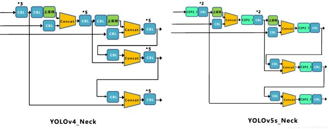
Yolov5和Yolov4的不同點(diǎn)在于,Yolov4的Neck中,采用的都是普通的卷積操作。而Yolov5的Neck結(jié)構(gòu)中,采用借鑒CSPNet設(shè)計(jì)的CSP2結(jié)構(gòu),加強(qiáng)網(wǎng)絡(luò)特征融合的能力。
1.4、輸出端的區(qū)別
1 Bounding box損失函數(shù)
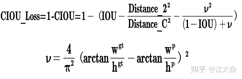
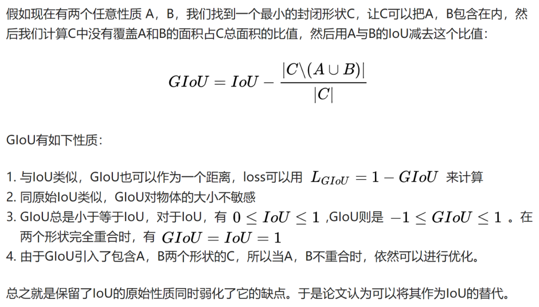
而Yolov4中采用CIOU_Loss作為目標(biāo)Bounding box的損失。而Yolov5中采用其中的GIOU_Loss做Bounding box的損失函數(shù)。
def compute_loss(p, targets, model):  # predictions, targets, model
    ft = torch.cuda.FloatTensor if p[0].is_cuda else torch.Tensor
    lcls, lbox, lobj = ft([0]), ft([0]), ft([0])
    tcls, tbox, indices, anchors = build_targets(p, targets, model)  # targets
    h = model.hyp  # hyperparameters
    red = 'mean'  # Loss reduction (sum or mean)

    # Define criteria
    BCEcls = nn.BCEWithLogitsLoss(pos_weight=ft([h['cls_pw']]), reduction=red)
    BCEobj = nn.BCEWithLogitsLoss(pos_weight=ft([h['obj_pw']]), reduction=red)

    # class label smoothing https://arxiv.org/pdf/1902.04103.pdf eqn 3
    cp, cn = smooth_BCE(eps=0.0)

    # focal loss
    g = h['fl_gamma']  # focal loss gamma
    if g > 0:
        BCEcls, BCEobj = FocalLoss(BCEcls, g), FocalLoss(BCEobj, g)

    # per output
    nt = 0  # targets
    for i, pi in enumerate(p):  # layer index, layer predictions
        b, a, gj, gi = indices[i]  # image, anchor, gridy, gridx
        tobj = torch.zeros_like(pi[..., 0])  # target obj

        nb = b.shape[0]  # number of targets
        if nb:
            nt += nb  # cumulative targets
            ps = pi[b, a, gj, gi]  # prediction subset corresponding to targets

            # GIoU
            pxy = ps[:, :2].sigmoid() * 2. - 0.5
            pwh = (ps[:, 2:4].sigmoid() * 2) ** 2 * anchors[i]
            pbox = torch.cat((pxy, pwh), 1)  # predicted box
            giou = bbox_iou(pbox.t(), tbox[i], x1y1x2y2=False, GIoU=True)  # giou(prediction, target)
            lbox += (1.0 - giou).sum() if red == 'sum' else (1.0 - giou).mean()  # giou loss

            # Obj
            tobj[b, a, gj, gi] = (1.0 - model.gr) + model.gr * giou.detach().clamp(0).type(tobj.dtype)  # giou ratio

            # Class
            if model.nc > 1:  # cls loss (only if multiple classes)
                t = torch.full_like(ps[:, 5:], cn)  # targets
                t[range(nb), tcls[i]] = cp
                lcls += BCEcls(ps[:, 5:], t)  # BCE

            # Append targets to text file
            # with open('targets.txt', 'a') as file:
            #     [file.write('%11.5g ' * 4 % tuple(x) + '\n') for x in torch.cat((txy[i], twh[i]), 1)]

        lobj += BCEobj(pi[..., 4], tobj)  # obj loss

    lbox *= h['giou']
    lobj *= h['obj']
    lcls *= h['cls']
    bs = tobj.shape[0]  # batch size
    if red == 'sum':
        g = 3.0  # loss gain
        lobj *= g / bs
        if nt:
            lcls *= g / nt / model.nc
            lbox *= g / nt

    loss = lbox + lobj + lcls
    return loss * bs, torch.cat((lbox, lobj, lcls, loss)).detach()
2 NMS非極大值抑制
Yolov4在DIOU_Loss的基礎(chǔ)上采用DIOU_NMS的方式,而Yolov5中采用加權(quán)NMS的方式。可以看出,采用DIOU_NMS,下方中間箭頭的黃色部分,原本被遮擋的摩托車也可以檢出。
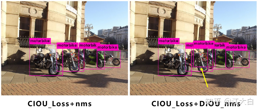
在同樣的參數(shù)情況下,將NMS中IOU修改成DIOU_NMS。對(duì)于一些遮擋重疊的目標(biāo),確實(shí)會(huì)有一些改進(jìn)。
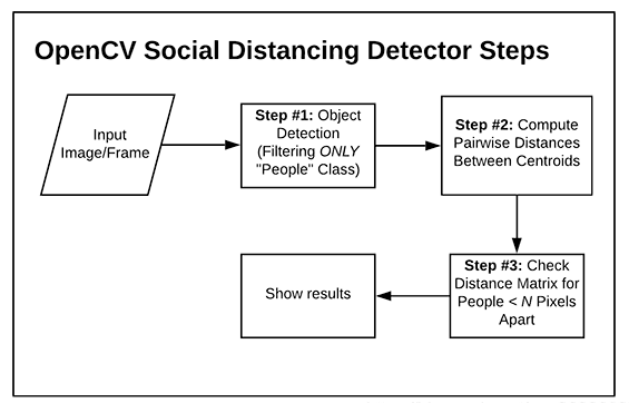
2、YOLOv5社交距離項(xiàng)目
yolov5檢測(cè)要檢測(cè)的視頻流中的所有人,然后再計(jì)算所有檢測(cè)到的人之間的相互“距離”,和現(xiàn)實(shí)生活中用“m”這樣的單位衡量距離不一樣的是,在計(jì)算機(jī)中,簡(jiǎn)單的方法是用檢測(cè)到的兩個(gè)人的質(zhì)心,也就是檢測(cè)到的目標(biāo)框的中心之間相隔的像素值作為計(jì)算機(jī)中的“距離”來衡量視頻中的人之間的距離是否超過安全距離。
構(gòu)建步驟:
使用目標(biāo)檢測(cè)算法檢測(cè)視頻流中的所有人,得到位置信息和質(zhì)心位置;
計(jì)算所有檢測(cè)到的人質(zhì)心之間的相互距離;
設(shè)置安全距離,計(jì)算每個(gè)人之間的距離對(duì),檢測(cè)兩個(gè)人之間的距離是否小于N個(gè)像素,小于則處于安全距離,反之則不處于。
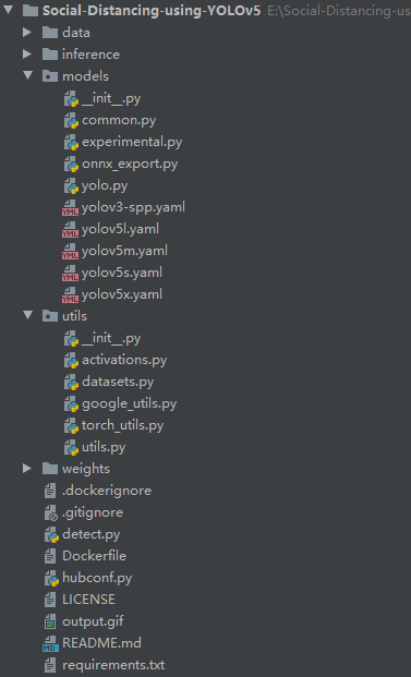
項(xiàng)目架構(gòu):
detect.py代碼注釋如下:
import argparse

from utils.datasets import *
from utils.utils import *


def detect(save_img=False):
    out, source, weights, view_img, save_txt, imgsz = \
        opt.output, opt.source, opt.weights, opt.view_img, opt.save_txt, opt.img_size
    webcam = source == '0' or source.startswith('rtsp') or source.startswith('http') or source.endswith('.txt')

    # Initialize
    device = torch_utils.select_device(opt.device)
    if os.path.exists(out):
        shutil.rmtree(out)  # delete output folder
    os.makedirs(out)  # make new output folder
    half = device.type != 'cpu'  # half precision only supported on CUDA

    # 下載模型
    google_utils.attempt_download(weights)
    # 加載權(quán)重
    model = torch.load(weights, map_location=device)['model'].float()
    # torch.save(torch.load(weights, map_location=device), weights)  # update model if SourceChangeWarning
    # model.fuse()
    # 設(shè)置模型為推理模式
    model.to(device).eval()
    if half:
        model.half()  # to FP16

    # Second-stage classifier
    classify = False
    if classify:
        modelc = torch_utils.load_classifier(name='resnet101', n=2)  # initialize
        modelc.load_state_dict(torch.load('weights/resnet101.pt', map_location=device)['model'])  # load weights
        modelc.to(device).eval()

    # 設(shè)置 Dataloader
    vid_path, vid_writer = None, None
    if webcam:
        view_img = True
        torch.backends.cudnn.benchmark = True  # set True to speed up constant image size inference
        dataset = LoadStreams(source, img_size=imgsz)
    else:
        save_img = True
        dataset = LoadImages(source, img_size=imgsz)

    # 獲取檢測(cè)類別的標(biāo)簽名稱
    names = model.names if hasattr(model, 'names') else model.modules.names
    # 定義顏色
    colors = [[random.randint(0, 255) for _ in range(3)] for _ in range(len(names))]

    # 開始推理
    t0 = time.time()
    # 初始化一張全為0的圖片
    img = torch.zeros((1, 3, imgsz, imgsz), device=device)
    _ = model(img.half() if half else img) if device.type != 'cpu' else None
    for path, img, im0s, vid_cap in dataset:
        img = torch.from_numpy(img).to(device)
        img = img.half() if half else img.float()  # uint8 to fp16/32
        img /= 255.0  # 0 - 255 to 0.0 - 1.0
        if img.ndimension() == 3:
            img = img.unsqueeze(0)

        # 預(yù)測(cè)結(jié)果
        t1 = torch_utils.time_synchronized()
        pred = model(img, augment=opt.augment)[0]

        # 使用NMS
        pred = non_max_suppression(pred, opt.conf_thres, opt.iou_thres, fast=True, classes=opt.classes, agnostic=opt.agnostic_nms)
        t2 = torch_utils.time_synchronized()

        # 進(jìn)行分類
        if classify:
            pred = apply_classifier(pred, modelc, img, im0s)

        people_coords = []

        # 處理預(yù)測(cè)得到的檢測(cè)目標(biāo)
        for i, det in enumerate(pred):
            if webcam:
                p, s, im0 = path[i], '%g: ' % i, im0s[i].copy()
            else:
                p, s, im0 = path, '', im0s

            save_path = str(Path(out) / Path(p).name)
            s += '%gx%g ' % img.shape[2:]  # print string
            gn = torch.tensor(im0.shape)[[1, 0, 1, 0]]  #  normalization gain whwh
            if det is not None and len(det):
                # 把boxes resize到im0的size
                det[:, :4] = scale_coords(img.shape[2:], det[:, :4], im0.shape).round()

                # 打印結(jié)果
                for c in det[:, -1].unique():
                    n = (det[:, -1] == c).sum()  # detections per class
                    s += '%g %ss, ' % (n, names[int(c)])  # add to string

                # 書寫結(jié)果
                for *xyxy, conf, cls in det:
                    if save_txt:
                        # xyxy2xywh ==> 把預(yù)測(cè)得到的坐標(biāo)結(jié)果[x1, y1, x2, y2]轉(zhuǎn)換為[x, y, w, h]其中 xy1=top-left, xy2=bottom-right
                        xywh = (xyxy2xywh(torch.tensor(xyxy).view(1, 4)) / gn).view(-1).tolist()  # normalized xywh
                        with open(save_path[:save_path.rfind('.')] + '.txt', 'a') as file:
                            file.write(('%g ' * 5 + '\n') % (cls, *xywh))  # label format

                    if save_img or view_img:  # Add bbox to image
                        label = '%s %.2f' % (names[int(cls)], conf)
                        if label is not None:
                            if (label.split())[0] == 'person':
                                # print(xyxy)
                                people_coords.append(xyxy)
                                # plot_one_box(xyxy, im0, line_thickness=3)
                                plot_dots_on_people(xyxy, im0)

            # 通過people_coords繪制people之間的連接線
            # 這里主要分為"Low Risk "和"High Risk"
            distancing(people_coords, im0, dist_thres_lim=(200, 250))

            # Print time (inference + NMS)
            print('%sDone. (%.3fs)' % (s, t2 - t1))

            # Stream results
            if view_img:
                cv2.imshow(p, im0)
                if cv2.waitKey(1) == ord('q'):  # q to quit
                    raise StopIteration

            # Save results (image with detections)
            if save_img:
                if dataset.mode == 'images':
                    cv2.imwrite(save_path, im0)
                else:
                    if vid_path != save_path:  # new video
                        vid_path = save_path
                        if isinstance(vid_writer, cv2.VideoWriter):
                            vid_writer.release()  # release previous video writer

                        fps = vid_cap.get(cv2.CAP_PROP_FPS)
                        w = int(vid_cap.get(cv2.CAP_PROP_FRAME_WIDTH))
                        h = int(vid_cap.get(cv2.CAP_PROP_FRAME_HEIGHT))
                        vid_writer = cv2.VideoWriter(save_path, cv2.VideoWriter_fourcc(*opt.fourcc), fps, (w, h))
                    vid_writer.write(im0)

    if save_txt or save_img:
        print('Results saved to %s' % os.getcwd() + os.sep + out)
        if platform == 'darwin':  # MacOS
            os.system('open ' + save_path)

    print('Done. (%.3fs)' % (time.time() - t0))


if __name__ == '__main__':
    parser = argparse.ArgumentParser()
    parser.add_argument('--weights', type=str, default='./weights/yolov5s.pt', help='model.pt path')
    parser.add_argument('--source', type=str, default='./inference/videos/', help='source')  # file/folder, 0 for webcam
    parser.add_argument('--output', type=str, default='./inference/output', help='output folder')  # output folder
    parser.add_argument('--img-size', type=int, default=640, help='inference size (pixels)')
    parser.add_argument('--conf-thres', type=float, default=0.4, help='object confidence threshold')
    parser.add_argument('--iou-thres', type=float, default=0.5, help='IOU threshold for NMS')
    parser.add_argument('--fourcc', type=str, default='mp4v', help='output video codec (verify ffmpeg support)')
    parser.add_argument('--device', default='0', help='cuda device, i.e. 0 or 0,1,2,3 or cpu')
    parser.add_argument('--view-img', action='store_true', help='display results')
    parser.add_argument('--save-txt', action='store_true', help='save results to *.txt')
    parser.add_argument('--classes', nargs='+', type=int, help='filter by class')
    parser.add_argument('--agnostic-nms', action='store_true', help='class-agnostic NMS')
    parser.add_argument('--augment', action='store_true', help='augmented inference')
    opt = parser.parse_args()
    opt.img_size = check_img_size(opt.img_size)
    print(opt)

    with torch.no_grad():
        detect()
參考
[1].https://zhuanlan.zhihu.com/p/172121380
[2].https://blog.csdn.net/weixin_45192980/article/details/108354169
[3].https://github.com/ultralytics/yoloV5
[4].https://github.com/Akbonline/Social-Distancing-using-YOLOv5
原文獲取方式,掃描下方二維碼
回復(fù)【YOLOV5-SD】即可獲取論文與源碼
聲明:轉(zhuǎn)載請(qǐng)說明出處
掃描下方二維碼關(guān)注【AI人工智能初學(xué)者】公眾號(hào),獲取更多實(shí)踐項(xiàng)目源碼和論文解讀,非常期待你我的相遇,讓我們以夢(mèng)為馬,砥礪前行!!!
點(diǎn)“在看”給我一朵小黃花唄![]()