一文快速入手:多實(shí)例學(xué)習(xí)
導(dǎo)讀
當(dāng)涉及到在醫(yī)學(xué)領(lǐng)域中應(yīng)用計算機(jī)視覺時,大多數(shù)任務(wù)涉及到:
(1) 用于診斷的圖像分類任務(wù)
(2) 識別和分離病變區(qū)域的分割任務(wù)
然而,在病理學(xué)癌癥檢測中,這并不總是可能的。獲取標(biāo)簽既費(fèi)時又費(fèi)力。此外,病理切片的分辨率最高可達(dá)200000 x 100000像素,并且它們不適合在內(nèi)存中進(jìn)行分類,因?yàn)槔纾琁mageNet僅使用224 x 224像素進(jìn)行訓(xùn)練。下采樣通常不是一個選項(xiàng),因?yàn)槲覀冊噲D檢測一個微小的區(qū)域,例如從300×300像素區(qū)域(圖1中的幾個點(diǎn))變化的癌區(qū)域。
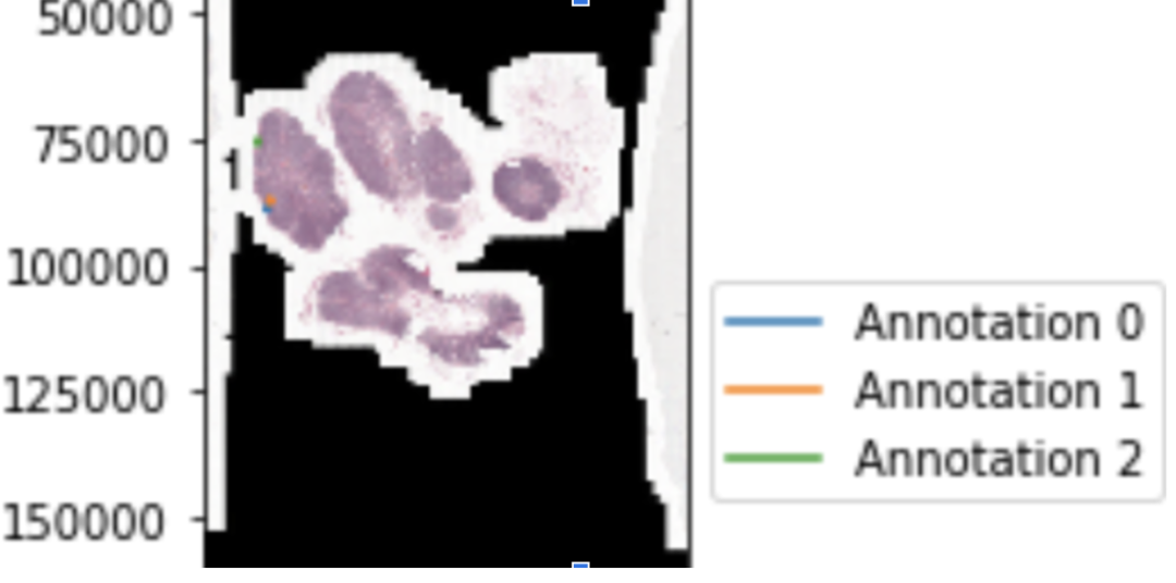
圖一:來自patient_ 004 _ node _ 004(cameloyon 17)的幻燈片
在這種情況下,我們可以使用多實(shí)例學(xué)習(xí)(Multiple Instance Learning),這是一種弱監(jiān)督學(xué)習(xí)方法,它采用一組包含許多實(shí)例的標(biāo)記包,而不是接收一組標(biāo)記實(shí)例。
假設(shè)我們有病理切片和每張切片的標(biāo)簽。因?yàn)槲覀儾荒茉谡麄€幻燈片上訓(xùn)練分類器,所以我們將每個幻燈片分成小塊,在GPU上一次只處理幾個小塊。然而,我們不知道每個圖塊的標(biāo)簽,因此我們需要多實(shí)例學(xué)習(xí)。在MIL框架中,幻燈片是“包”,切片是“實(shí)例”。通過使用它,我們能夠節(jié)省標(biāo)記工作,并利用弱標(biāo)記數(shù)據(jù)。
當(dāng)我們有患者的病理切片時,我們希望預(yù)測大切片是否包含癌細(xì)胞,或者縮小患者是否有惡性細(xì)胞,多實(shí)例學(xué)習(xí)是一個很好的選擇,因?yàn)獒t(yī)生不需要分割單個細(xì)胞或標(biāo)記每個切片。只有整張幻燈片需要標(biāo)簽。
一般來說,多實(shí)例學(xué)習(xí)可以處理分類問題、回歸問題、排序問題和聚類問題,但我們這里主要關(guān)注分類問題。
在這篇文章中,我將通過一個基于 MNIST 數(shù)據(jù)集的簡單示例來解釋 MIL 如何工作。如果你不熟悉 MNIST 數(shù)據(jù)集,這里有一個[關(guān)于 MNIST 數(shù)據(jù)集](https://www.kaggle.com/ngbolin/mnist-dataset-digit-recognizer)的[Kaggle 競賽](https://www.kaggle.com/ngbolin/mnist-dataset-digit-recognizer)的鏈接,你可以看看。
MNIST數(shù)據(jù)集簡介
MNIST數(shù)據(jù)集是一個手寫數(shù)字的大型數(shù)據(jù)庫,每個圖像都有一個從0到9的標(biāo)簽。它有6萬張圖像的訓(xùn)練集和1萬張圖像的測試集。每個的尺寸是28 x 28的灰度圖。
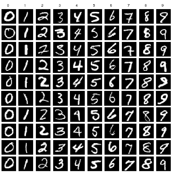
圖 2: Minst 手寫分類數(shù)據(jù)集
多實(shí)例學(xué)習(xí)的問題簡述
一個袋子里的xi每個實(shí)例都有一個標(biāo)簽yi。我們將包的標(biāo)簽定義為:
Y = 1,如果存在 yi ==1
Y = 0,如果對于每個yi,yi == 0
在MNIST數(shù)據(jù)集上應(yīng)用多元線性回歸的流程
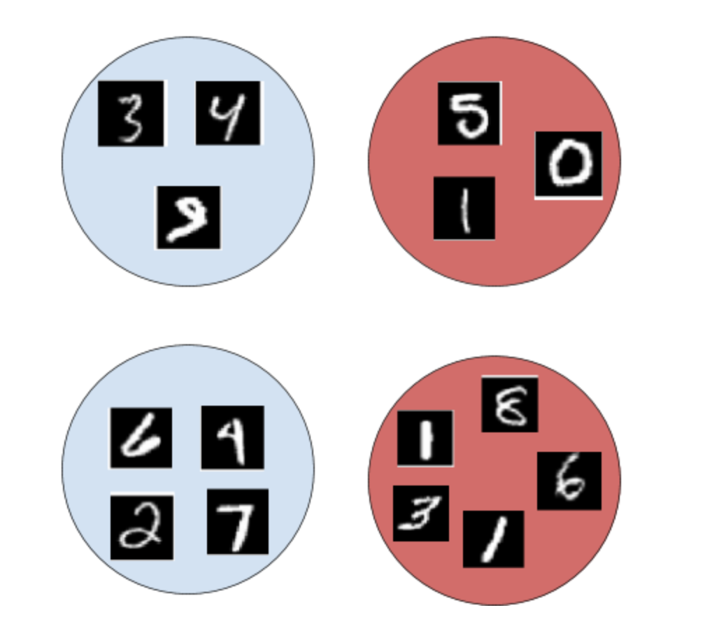
圖 3:袋子和實(shí)例標(biāo)簽
我們將每個圖像隨機(jī)放入一個包中,每個包包含 3 到 7 個實(shí)例。為了節(jié)省內(nèi)存,我們使用索引來表示圖像(如下圖)。
def data_generation(instance_index_label: List[Tuple]) -> List[Dict]:"""bags: {key1: [ind1, ind2, ind3],key2: [ind1, ind2, ind3, ind4, ind5],... }bag_lbls:{key1: 0,key2: 1,... }"""bag_size = np.random.randint(3,7,size=len(instance_index_label)//5)data_cp = copy.copy(instance_index_label)np.random.shuffle(data_cp)bags = {}bags_per_instance_labels = {}bags_labels = {}for bag_ind, size in enumerate(bag_size):bags[bag_ind] = []bags_per_instance_labels[bag_ind] = []try:for _ in range(size):inst_ind, lbl = data_cp.pop()bags[bag_ind].append(inst_ind)# simplfy, just use a temporary variable instead of bags_per_instance_labelsbags_per_instance_labels[bag_ind].append(lbl)bags_labels[bag_ind] = bag_label_from_instance_labels(bags_per_instance_labels[bag_ind])except:breakreturn bags, bags_labels
生成包標(biāo)簽:
def bag_label_from_instance_labels(instance_labels):return int(any(((x==1) for x in instance_labels)))
第 2 步:對 MNIST 數(shù)據(jù)集的 2 個部分進(jìn)行預(yù)訓(xùn)練
1. 構(gòu)造一個2D卷積神經(jīng)網(wǎng)絡(luò),kernel_size=(7, 7), stride=(2, 2), padding=(3, 3)
2. 訓(xùn)練 5 個 epoch,批大小為 256
3. 保存模型
import torchfrom torchvision.models.resnet import ResNet, BasicBlockclass MnistResNet(ResNet):def __init__(self):super(MnistResNet, self).__init__(BasicBlock, [2, 2, 2, 2], num_classes=10)self.conv1 = torch.nn.Conv2d(1, 64, kernel_size=(7, 7), stride=(2, 2), padding=(3, 3), bias=False)def forward(self, x):return torch.softmax(super(MnistResNet, self).forward(x), dim=-1)
第 3 步:加載預(yù)訓(xùn)練模型并從最后一層提取特征
1. 將其余數(shù)據(jù)拆分為訓(xùn)練、驗(yàn)證和測試集
2. 獲取訓(xùn)練、驗(yàn)證和測試集的特征
3. 獲取 bag_indices 和 bag_labels
4. 使用基于索引的特征映射 bag_indices 并創(chuàng)建 bag_features
為了擺脫最后一層:
model = MnistResNet()model.load_state_dict(torch.load('mnist_state.pt'))body = nn.Sequential(*list(model.children()))# extract the last layermodel = body[:9]# the model we will usemodel.eval()
提取特征:
下面的代碼展示了我們?nèi)绾螐臄?shù)據(jù)生成函數(shù)中獲取包索引和包特征:
bag_indices, bag_labels = data_generation(instance_index_label)bag_features = {kk: torch.Tensor(feature_array[inds]) for kk, inds in bag_indices.items()}
袋子索引、袋子標(biāo)簽和袋子特征如下所示:
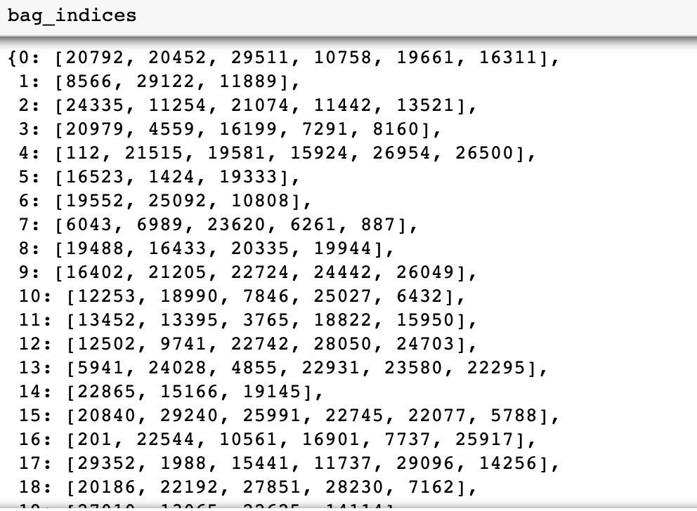
圖 7:帶圖像索引的袋子索引
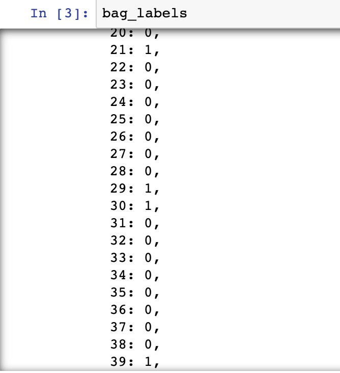
圖 8:袋子標(biāo)簽
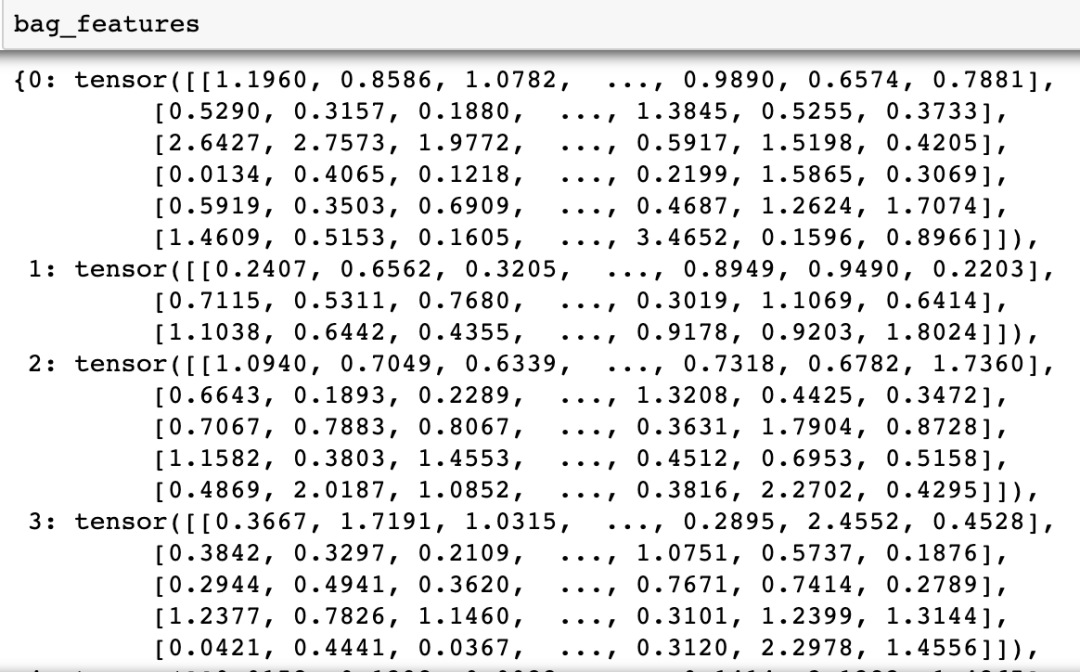
圖 9:袋子特征
第 4 步:在 bag_features 和 bag_labels 上訓(xùn)練 MIL 模型并在測試集上進(jìn)行評估
由于每個包都有不同數(shù)量的實(shí)例,我們需要在將張量放入模型之前將它們填充到相同的大小。
多實(shí)例學(xué)習(xí)模型:
該算法執(zhí)行三個步驟。它們中的任何一個都可以是固定函數(shù)或可優(yōu)化函數(shù)(神經(jīng)網(wǎng)絡(luò)):
1. 將實(shí)例轉(zhuǎn)換為低維嵌入。(固定的)
2. 通過置換不變聚合函數(shù)傳遞嵌入。(可優(yōu)化)
3. 轉(zhuǎn)化為包概率。(可優(yōu)化)
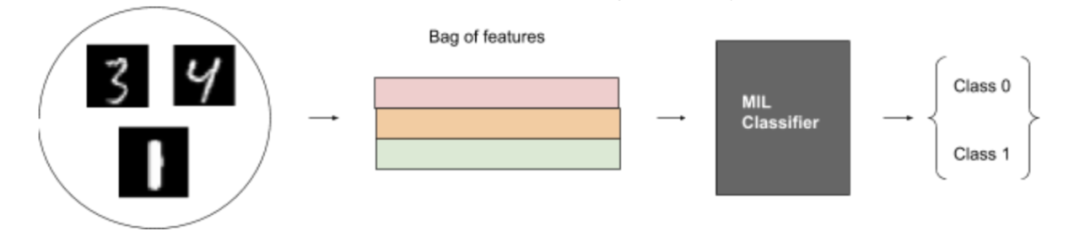
圖 9:MIL-MNIST 玩具數(shù)據(jù)集上的 MIL 圖
一般來說,工作流程如下:
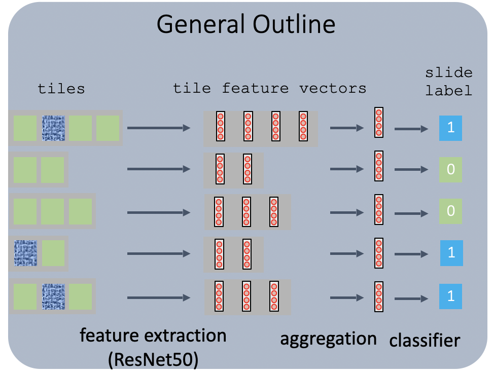
圖 10:病理切片上的 MIL 算法框架圖(參見參考文獻(xiàn) #5)
為簡單起見,我們將步驟 1 固定為固定。對于第 2 步,雖然我們?nèi)匀豢梢允褂霉潭ê瘮?shù),例如 max 或 mean,但為了啟用可以通過反向傳播端到端學(xué)習(xí)的參數(shù)優(yōu)化,我們使用神經(jīng)網(wǎng)絡(luò)作為聚合函數(shù)。對于第 3 步,我們還希望使用反向傳播來優(yōu)化參數(shù)。
1. 線性層和 LeakyReLu
class NoisyAnd(torch.nn.Module):def __init__(self, a=10, dims=[1,2]):super(NoisyAnd, self).__init__()# self.output_dim = output_dimself.a = aself.b = torch.nn.Parameter(torch.tensor(0.01))self.dims =dimsself.sigmoid = nn.Sigmoid()def forward(self, x):# h_relu = self.linear1(x).clamp(min=0)mean = torch.mean(x, self.dims, True)res = (self.sigmoid(self.a * (mean - self.b)) - self.sigmoid(-self.a * self.b)) / (self.sigmoid(self.a * (1 - self.b)) - self.sigmoid(-self.a * self.b))return resclass NN(torch.nn.Module):def __init__(self, n=512, n_mid = 1024,n_out=1, dropout=0.2,scoring = None,):super(NN, self).__init__()self.linear1 = torch.nn.Linear(n, n_mid)self.non_linearity = torch.nn.LeakyReLU()self.linear2 = torch.nn.Linear(n_mid, n_out)self.dropout = torch.nn.Dropout(dropout)if scoring:self.scoring = scoringelse:self.scoring = torch.nn.Softmax() if n_out>1 else torch.nn.Sigmoid()def forward(self, x):z = self.linear1(x)z = self.non_linearity(z)z = self.dropout(z)z = self.linear2(z)y_pred = self.scoring(z)return y_predclass LogisticRegression(torch.nn.Module):def __init__(self, n=512, n_out=1):super(LogisticRegression, self).__init__()self.linear = torch.nn.Linear(n, n_out)self.scoring = torch.nn.Softmax() if n_out>1 else torch.nn.Sigmoid()def forward(self, x):z = self.linear(x)y_pred = self.scoring(z)return y_preddef regularization_loss(params,reg_factor = 0.005,reg_alpha = 0.5):params = [pp for pp in params if len(pp.shape)>1]l1_reg = nn.L1Loss()l2_reg = nn.MSELoss()loss_reg =0for pp in params:loss_reg+=reg_factor*((1-reg_alpha)*l1_reg(pp, target=torch.zeros_like(pp)) +\reg_alpha*l2_reg(pp, target=torch.zeros_like(pp)))return loss_reg
注意:我們設(shè)置 n = 7*512,其中 7 是一個包中的實(shí)例數(shù),512 是每個特征的大小。
2. 聚合函數(shù):AttensionSoftmax
class SoftMaxMeanSimple(torch.nn.Module):def __init__(self, n, n_inst, dim=0):"""if dim==1:given a tensor `x` with dimensions [N * M],where M -- dimensionality of the featur vector(number of features per instance)N -- number of instancesinitialize with `AggModule(M)`returns:- weighted result: [M]- gate: [N]if dim==0:..."""super(SoftMaxMeanSimple, self).__init__()self.dim = dimself.gate = torch.nn.Softmax(dim=self.dim)self.mdl_instance_transform = nn.Sequential(nn.Linear(n, n_inst),nn.LeakyReLU(),nn.Linear(n_inst, n),nn.LeakyReLU(),)def forward(self, x):z = self.mdl_instance_transform(x)if self.dim==0:z = z.view((z.shape[0],1)).sum(1)elif self.dim==1:z = z.view((1, z.shape[1])).sum(0)gate_ = self.gate(z)res = torch.sum(x* gate_, self.dim)return res, gate_class AttentionSoftMax(torch.nn.Module):def __init__(self, in_features = 3, out_features = None):"""given a tensor `x` with dimensions [N * M],where M -- dimensionality of the featur vector(number of features per instance)N -- number of instancesinitialize with `AggModule(M)`returns:- weighted result: [M]- gate: [N]"""super(AttentionSoftMax, self).__init__()self.otherdim = ''if out_features is None:out_features = in_featuresself.layer_linear_tr = nn.Linear(in_features, out_features)self.activation = nn.LeakyReLU()self.layer_linear_query = nn.Linear(out_features, 1)def forward(self, x):keys = self.layer_linear_tr(x)keys = self.activation(keys)attention_map_raw = self.layer_linear_query(keys)[...,0]attention_map = nn.Softmax(dim=-1)(attention_map_raw)result = torch.einsum(f'{self.otherdim}i,{self.otherdim}ij->{self.otherdim}j', attention_map, x)return result, attention_map
3. 中間以LeakyReLu為激活函數(shù),dropout,sigmoid為最終激活函數(shù)的神經(jīng)網(wǎng)絡(luò):
class MIL_NN(torch.nn.Module):def __init__(self, n=512,n_mid=1024,n_classes=1,dropout=0.1,agg = None,scoring=None,):super(MIL_NN, self).__init__()self.agg = agg if agg is not None else AttentionSoftMax(n)if n_mid == 0:self.bag_model = LogisticRegression(n, n_classes)else:self.bag_model = NN(n, n_mid, n_classes, dropout=dropout, scoring=scoring)def forward(self, bag_features, bag_lbls=None):"""bag_feature is an aggregated vector of 512 featuresbag_att is a gate vector of n_inst instancesbag_lbl is a vector a labelsfigure out batches"""bag_feature, bag_att, bag_keys = list(zip(*[list(self.agg(ff.float())) + [idx]for idx, ff in (bag_features.items())]))bag_att = dict(zip(bag_keys, [a.detach().cpu() for a in bag_att]))bag_feature_stacked = torch.stack(bag_feature)y_pred = self.bag_model(bag_feature_stacked)return y_pred, bag_att, bag_keys
4. 優(yōu)化器:SGD
5. 損失函數(shù):BCELoss
6. 準(zhǔn)確度:~0.99
結(jié)論
我們使用 MIL 在 MNIST 數(shù)據(jù)集上獲得了大約 0.99 的準(zhǔn)確率,這是一個令人滿意的結(jié)果。如果我們愿意,我們可以使用更復(fù)雜的聚合函數(shù)作為我們的中間轉(zhuǎn)換,并構(gòu)建更復(fù)雜的 NN 模型用于最終轉(zhuǎn)換到包級別。結(jié)果還表明,MIL 是一個很好的工具,可以節(jié)省標(biāo)記工作并利用弱標(biāo)記數(shù)據(jù)。
Jupyter 筆記本演示鏈接:
https://github.com/lsheng23/Practicum/blob/master/MIL_MNIST/end_to_end_mnist_MIL.ipynb 點(diǎn)藍(lán)色字關(guān)注“機(jī)器學(xué)習(xí)算法工程師”
設(shè)為星標(biāo),干貨直達(dá)!
推薦閱讀
谷歌AI用30億數(shù)據(jù)訓(xùn)練了一個20億參數(shù)Vision Transformer模型,在ImageNet上達(dá)到新的SOTA!
"未來"的經(jīng)典之作ViT:transformer is all you need!
PVT:可用于密集任務(wù)backbone的金字塔視覺transformer!
漲點(diǎn)神器FixRes:兩次超越ImageNet數(shù)據(jù)集上的SOTA
不妨試試MoCo,來替換ImageNet上pretrain模型!
機(jī)器學(xué)習(xí)算法工程師
一個用心的公眾號