
【深度學(xué)習(xí)】實戰(zhàn)教程 | 車道線檢測項目實戰(zhàn),霍夫變換 & 新方法 Spatial CNN
此文按照這樣的邏輯進行撰寫。分享機器學(xué)習(xí)、計算機視覺的基礎(chǔ)知識,接著我們以一個實際的項目,帶領(lǐng)大家自己動手實踐。最后,分享更多學(xué)習(xí)資料、進階項目實戰(zhàn),這部分屬于我CSDN上的專欄,最后會按照順序給出相應(yīng)的鏈接,供大家選擇學(xué)習(xí)。
理論篇:算法基礎(chǔ)(可選擇后看)
本專欄所涉及的項目所需機器學(xué)習(xí)/圖像處理知識并不深入,但我之前在CSDN也開設(shè)了《機器學(xué)習(xí)算法講解與Python實現(xiàn)》和《計算機視覺前沿論文研讀》兩個專欄。一個更偏算法理論,一個則關(guān)注于計算機視覺頂會的前沿論文成果,解讀新的方法和Idea。
《機器學(xué)習(xí)算法講解與Python實現(xiàn)》
專欄鏈接 https://blog.csdn.net/charmve/category_9657673.html
《計算機視覺前沿論文研讀》
專欄鏈接 https://blog.csdn.net/charmve/category_10281912_2.html
計算機視覺實戰(zhàn) | 練手項目,開放源碼

專欄鏈接 https://blog.csdn.net/charmve/category_10595130.html
實戰(zhàn)案例(本文核心)
為什么說上述兩個關(guān)于機器學(xué)習(xí)基礎(chǔ)的專欄可以跳過?我的考慮是,如果對于機器學(xué)習(xí)剛?cè)腴T的同學(xué),直接上手算法理論,公式推導(dǎo)很容易消耗我們的學(xué)習(xí)熱情和積極性;另外,對于一些非研究人員,我們做項目的直接目的是能跑出實驗結(jié)果,一開始就帶著工程思維去學(xué)習(xí),效率會很高,學(xué)習(xí)的積極性也容易保持。這也是當(dāng)前很多模型都已在相應(yīng)的深度學(xué)習(xí)框架下集成了模塊和函數(shù)庫。而對于剩余一部分,可能需要重新回顧上述兩章內(nèi)容,深入理解算法原理,對算法性能的提升、模型的壓縮優(yōu)化都是很有必要的。
在某些情況下,直接調(diào)用已經(jīng)搭好的模型可能是非常方便且有效的,比如Caffe、TensorFlow工具箱,但這些工具箱需要的硬件資源比較多,不利于初學(xué)者實踐和理解。因此,為了更好的理解并掌握相關(guān)知識,最好是能夠自己編程實踐下。本文將展示計算機時如何識別車道線的。
Waymo的自動駕駛出租車服務(wù)本月已經(jīng)上路,但是自動駕駛汽車是如何工作的?道路上的線條向駕駛員指示了車道所在的位置,并作為相應(yīng)方向引導(dǎo)車輛的方向的指導(dǎo)性參考,并約定了車輛代理如何在道路上和諧地行駛。 同樣,識別和跟蹤車道的能力對于開發(fā)無人駕駛車輛算法至關(guān)重要。
在本教程中,我們將學(xué)習(xí)如何使用計算機視覺技術(shù)來編寫車道線實時檢測程序。我們將通過兩種不同的方法來完成這項任務(wù),從實際的算法編寫流程帶領(lǐng)大家從實現(xiàn)到優(yōu)化的過程。
方法1:霍夫變換
大多數(shù)車道的設(shè)計都相對簡單明了,不僅可以鼓勵交通秩序井然,還可以使駕駛員更輕松地以恒定的速度駕駛車輛。因此,我們的直觀方法可能是首先通過邊緣檢測和特征提取技術(shù)來檢測攝像機饋送中的突出直線。我們將使用OpenCV(一種計算機視覺算法的開源庫)來實現(xiàn)。下圖是我們算法流程的概述。

1.設(shè)置環(huán)境
如果您尚未安裝OpenCV,請打開“終端”并運行以安裝它:
pip install opencv-python
現(xiàn)在,通過運行以下命令來clone本項目的實踐代碼:
git clone https://github.com/Charmve/Awesome-Lane-Detection.git
接下來,進入lane-detector文件夾
cd lane-detector
使用文本編輯器打開detector.py。我們將在此Python文件中編寫本節(jié)的所有代碼。
2.處理視頻
我們將以10毫秒為間隔的一系列連續(xù)幀(圖像)輸入用于車道檢測的示例視頻。我們也可以隨時按“ q”鍵退出程序。
import cv2 as cv# The video feed is read in as a VideoCapture objectcap = cv.VideoCapture("input.mp4")while (cap.isOpened()):# ret = a boolean return value from getting the frame, frame = the current frame being projected in the videoret, frame = cap.read()# Frames are read by intervals of 10 milliseconds. The programs breaks out of the while loop when the user presses the 'q' keyif cv.waitKey(10) & 0xFF == ord('q'):break# The following frees up resources and closes all windowscap.release()cv.destroyAllWindows()
3.應(yīng)用Canny Detector
Canny Detector是為快速實時邊緣檢測而優(yōu)化的多階段算法。該算法的基本目標(biāo)是檢測亮度的急劇變化(大梯度),例如從白色到黑色的變化,并在給定一組閾值的情況下將它們定義為邊緣。
Canny算法有四個主要階段:
A.降噪
與所有邊緣檢測算法一樣,噪聲是一個關(guān)鍵問題,通常會導(dǎo)致錯誤檢測。應(yīng)用5x5高斯濾波器對圖像進行卷積(平滑),以降低檢測器對噪聲的敏感度。這是通過使用正態(tài)分布數(shù)的內(nèi)核(在本例中為5x5內(nèi)核)在整個圖像上運行來完成的,將每個像素值設(shè)置為等于其相鄰像素的加權(quán)平均值。
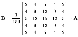
5x5高斯核,星號“*”表示卷積運算。
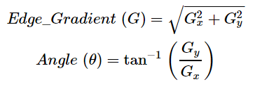
B.強度梯度
然后使用平滑化的圖像沿x軸和y軸應(yīng)用Sobel,Roberts或Prewitt內(nèi)核(OpenCV中使用了Sobel),以檢測邊緣是水平,垂直還是對角線。(在這里你可以先不用管Sobel,Roberts或Prewitt內(nèi)核,他們是什么。)
Sobel內(nèi)核,用于計算水平和垂直方向的一階導(dǎo)數(shù)
C.非最大抑制
非最大抑制可應(yīng)用于削“薄(thin)”并有效銳化邊緣。對于每個像素,檢查該值是否在先前計算的漸變方向上是局部最大值。

三點非最大抑制
A在具有垂直方向的邊緣上。由于梯度垂直于邊緣方向,因此將B和C的像素值與A的像素值進行比較,以確定A是否為局部最大值。如果A是局部最大值,則對下一個點測試非最大值抑制;否則,將A的像素值設(shè)置為零,并抑制A。
D.磁滯閾值
在非最大抑制之后,確認強像素位于邊緣的最終貼圖中。但是,應(yīng)進一步分析弱像素,以確定其構(gòu)成為邊緣還是噪聲。應(yīng)用兩個預(yù)定義的minVal和maxVal閾值,我們設(shè)置強度梯度大于maxVal的任何像素為邊緣,強度梯度小于minVal的任何像素都不為邊緣并丟棄。如果亮度梯度介于minVal和maxVal之間的像素連接到強度梯度大于maxVal的像素,則僅將其視為邊緣。

圖1 兩行磁滯閾值示例
邊緣A高于maxVal,因此被視為邊緣。邊緣B在maxVal和minVal之間,但未連接到maxVal以上的任何邊緣,因此將其丟棄。邊緣C在maxVal和minVal之間,并連接到邊緣A,即maxVal之上的邊緣,因此被視為邊緣。
對于該算法流程,我們首先要對視頻幀進行灰度處理,因為我們只需要用于檢測邊緣的亮度通道,并應(yīng)用5 x 5高斯模糊來減少噪聲以減少虛假邊緣。
# import cv2 as cvdef do_canny(frame):# Converts frame to grayscale because we only need the luminance channel for detecting edges - less computationally expensivegray = cv.cvtColor(frame, cv.COLOR_RGB2GRAY)# Applies a 5x5 gaussian blur with deviation of 0 to frame - not mandatory since Canny will do this for usblur = cv.GaussianBlur(gray, (5, 5), 0)# Applies Canny edge detector with minVal of 50 and maxVal of 150canny = cv.Canny(blur, 50, 150)return canny# cap = cv.VideoCapture("input.mp4")# while (cap.isOpened()):# ret, frame = cap.read()canny = do_canny(frame)# if cv.waitKey(10) & 0xFF == ord('q'):# break# cap.release()# cv.destroyAllWindows()
4.分割車道區(qū)域
我們將手工制作一個三角形的蒙版,以分割車道區(qū)域,并丟棄車架中無關(guān)的區(qū)域,以提高我們后期的效率。 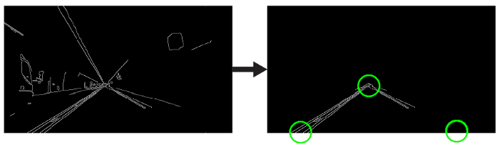 三角形遮罩將由三個坐標(biāo)定義,用綠色圓圈表示。
# import cv2 as cvimport numpy as npimport matplotlib.pyplot as plt# def do_canny(frame):# gray = cv.cvtColor(frame, cv.COLOR_RGB2GRAY)# blur = cv.GaussianBlur(gray, (5, 5), 0)# canny = cv.Canny(blur, 50, 150)# return cannydef do_segment(frame):# Since an image is a multi-directional array containing the relative intensities of each pixel in the image, we can use frame.shape to return a tuple: [number of rows, number of columns, number of channels] of the dimensions of the frame# frame.shape[0] give us the number of rows of pixels the frame has. Since height begins from 0 at the top, the y-coordinate of the bottom of the frame is its heightheight = frame.shape[0]# Creates a triangular polygon for the mask defined by three (x, y) coordinatespolygons = np.array([height), (800, height), (380, 290)]])# Creates an image filled with zero intensities with the same dimensions as the framemask = np.zeros_like(frame)# Allows the mask to be filled with values of 1 and the other areas to be filled with values of 0polygons, 255)# A bitwise and operation between the mask and frame keeps only the triangular area of the framesegment = cv.bitwise_and(frame, mask)return segment# cap = cv.VideoCapture("input.mp4")# while (cap.isOpened()):# ret, frame = cap.read()# canny = do_canny(frame)# First, visualize the frame to figure out the three coordinates defining the triangular maskplt.imshow(frame)plt.show()segment = do_segment(canny)# if cv.waitKey(10) & 0xFF == ord('q'):# break# cap.release()# cv.destroyAllWindows()
5.霍夫變換
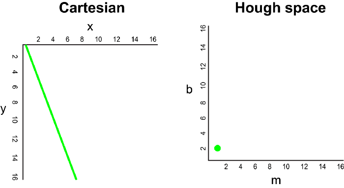
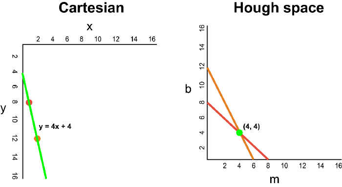
在笛卡爾坐標(biāo)系中,通過將y相對于x繪制,可以將一條直線表示為y = mx + b。但是,我們也可以通過將b相對于m繪制,將該線表示為Hough Space 霍夫空間中的單個點。例如,在霍夫空間中,具有等式y(tǒng) = 2x +1的線可以表示為(2,1)。
現(xiàn)在,如果要代替直線,我們必須在笛卡爾坐標(biāo)系中繪制一個點。有許多可能的線可以通過此點,每條線的參數(shù)m和b的值均不同。例如,可以通過y = 2x + 8,y = 3x + 6,y = 4x + 4,y = 5x + 2,y = 6x來傳遞 (2,12) 點。這些可能的線可以在Hough空間中繪制為(2,8),(3,6),(4,4),(5,2),(6,0)。請注意,這會在Hough空間中針對b坐標(biāo)生成一條m線。
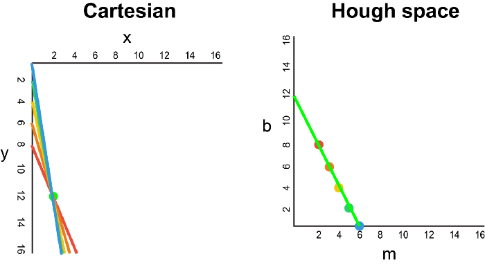
每當(dāng)我們看到笛卡爾坐標(biāo)系中的一系列點并且知道這些點由某條線連接時,我們就可以通過首先將笛卡爾坐標(biāo)系中的每個點繪制到Hough空間中的對應(yīng)線上,然后找到該線的方程。在霍夫空間中找到交點。霍夫空間中的交點表示連續(xù)通過序列中所有點的m和b值。
由于通過Canny Detector的幀可以簡單地解釋為代表我們圖像空間中邊緣的一系列白點,因此我們可以應(yīng)用相同的技術(shù)來識別這些點中的哪些連接到同一條線上,以及它們是否已連接,它的等式是什么,以便我們可以在框架上繪制這條線。
為了簡化說明,我們使用笛卡爾坐標(biāo)來對應(yīng)霍夫空間。但是,這種方法存在一個數(shù)學(xué)缺陷:當(dāng)直線垂直時,漸變?yōu)闊o窮大,無法在霍夫空間中表示。 為了解決這個問題,我們將使用極坐標(biāo)。除了在霍夫空間中將m相對于b繪制之外,該過程仍然相同,我們將r相對于θ進行繪制。
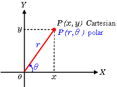
例如,對于極坐標(biāo)系上x = 8和y = 6,x = 4和y = 9,x = 12和y = 3的點,我們可以繪制相應(yīng)的霍夫空間。
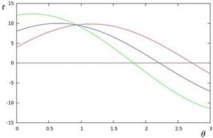
我們看到,霍夫空間中的線在θ= 0.925和r = 9.6處相交。由于極坐標(biāo)系中的一條線由r =xcosθ+ysinθ給出,因此我們可以得出一條穿過所有這些點的單線定義為9.6 = xcos0.925 + ysin0.925。
通常,在霍夫空間中相交的曲線越多,意味著該相交所代表的線對應(yīng)于更多的點。對于我們的實現(xiàn),我們將在霍夫空間中定義一個最小閾值交叉點以檢測一條線。因此,霍夫變換基本上可以跟蹤幀中每個點的霍夫空間相交。如果交叉點的數(shù)量超過定義的閾值,我們將確定一條具有相應(yīng)θ和r參數(shù)的線。
我們應(yīng)用霍夫變換來識別兩條直線,這將是我們的左右車道邊界。
import cv2 as cvimport numpy as np# import matplotlib.pyplot as plt# def do_canny(frame):gray = cv.cvtColor(frame, cv.COLOR_RGB2GRAY)blur = cv.GaussianBlur(gray, (5, 5), 0)canny = cv.Canny(blur, 50, 150)return canny# def do_segment(frame):height = frame.shape[0]polygons = np.array([[(0, height), (800, height), (380, 290)]])mask = np.zeros_like(frame)cv.fillPoly(mask, polygons, 255)segment = cv.bitwise_and(frame, mask)return segment# cap = cv.VideoCapture("input.mp4")while (cap.isOpened()):ret, frame = cap.read()canny = do_canny(frame)# plt.imshow(frame)# plt.show()segment = do_segment(canny)# cv.HoughLinesP(frame, distance resolution of accumulator in pixels (larger = less precision), angle resolution of accumulator in radians (larger = less precision), threshold of minimum number of intersections, empty placeholder array, minimum length of line in pixels, maximum distance in pixels between disconnected lines)hough = cv.HoughLinesP(segment, 2, np.pi / 180, 100, np.array([]), minLineLength = 100, maxLineGap = 50)# if cv.waitKey(10) & 0xFF == ord('q'):break# cap.release()cv.destroyAllWindows()
6.可視化
車道顯示為兩個淺綠色,線性擬合的多項式,這些多項式將覆蓋在我們的輸入框中。
# import cv2 as cv# import numpy as np# # import matplotlib.pyplot as plt# def do_canny(frame):# gray = cv.cvtColor(frame, cv.COLOR_RGB2GRAY)# blur = cv.GaussianBlur(gray, (5, 5), 0)# canny = cv.Canny(blur, 50, 150)# return canny# def do_segment(frame):# height = frame.shape[0]# polygons = np.array([# [(0, height), (800, height), (380, 290)]# ])# mask = np.zeros_like(frame)# cv.fillPoly(mask, polygons, 255)# segment = cv.bitwise_and(frame, mask)# return segmentdef calculate_lines(frame, lines):# Empty arrays to store the coordinates of the left and right linesleft = []right = []# Loops through every detected linefor line in lines:# Reshapes line from 2D array to 1D arrayy1, x2, y2 = line.reshape(4)# Fits a linear polynomial to the x and y coordinates and returns a vector of coefficients which describe the slope and y-interceptparameters = np.polyfit((x1, x2), (y1, y2), 1)slope = parameters[0]y_intercept = parameters[1]# If slope is negative, the line is to the left of the lane, and otherwise, the line is to the right of the laneif slope < 0:y_intercept))else:y_intercept))# Averages out all the values for left and right into a single slope and y-intercept value for each lineleft_avg = np.average(left, axis = 0)right_avg = np.average(right, axis = 0)# Calculates the x1, y1, x2, y2 coordinates for the left and right linesleft_line = calculate_coordinates(frame, left_avg)right_line = calculate_coordinates(frame, right_avg)return np.array([left_line, right_line])def calculate_coordinates(frame, parameters):intercept = parameters# Sets initial y-coordinate as height from top down (bottom of the frame)y1 = frame.shape[0]# Sets final y-coordinate as 150 above the bottom of the framey2 = int(y1 - 150)# Sets initial x-coordinate as (y1 - b) / m since y1 = mx1 + bx1 = int((y1 - intercept) / slope)# Sets final x-coordinate as (y2 - b) / m since y2 = mx2 + bx2 = int((y2 - intercept) / slope)return np.array([x1, y1, x2, y2])def visualize_lines(frame, lines):# Creates an image filled with zero intensities with the same dimensions as the framelines_visualize = np.zeros_like(frame)# Checks if any lines are detectedif lines is not None:for x1, y1, x2, y2 in lines:# Draws lines between two coordinates with green color and 5 thickness(x1, y1), (x2, y2), (0, 255, 0), 5)return lines_visualize# cap = cv.VideoCapture("input.mp4")# while (cap.isOpened()):# ret, frame = cap.read()# canny = do_canny(frame)# # plt.imshow(frame)# # plt.show()# segment = do_segment(canny)# hough = cv.HoughLinesP(segment, 2, np.pi / 180, 100, np.array([]), minLineLength = 100, maxLineGap = 50)# Averages multiple detected lines from hough into one line for left border of lane and one line for right border of lanelines = calculate_lines(frame, hough)# Visualizes the lineslines_visualize = visualize_lines(frame, lines)# Overlays lines on frame by taking their weighted sums and adding an arbitrary scalar value of 1 as the gamma argumentoutput = cv.addWeighted(frame, 0.9, lines_visualize, 1, 1)# Opens a new window and displays the output frameoutput)# if cv.waitKey(10) & 0xFF == ord('q'):# break# cap.release()# cv.destroyAllWindows()
現(xiàn)在,打開Terminal并運行pythondetector.py來測試您的簡單車道檢測器!如果您錯過任何代碼,這是帶有注釋的完整解決方案:
import cv2 as cvimport numpy as np# import matplotlib.pyplot as pltdef do_canny(frame):# Converts frame to grayscale because we only need the luminance channel for detecting edges - less computationally expensivegray = cv.cvtColor(frame, cv.COLOR_RGB2GRAY)# Applies a 5x5 gaussian blur with deviation of 0 to frame - not mandatory since Canny will do this for usblur = cv.GaussianBlur(gray, (5, 5), 0)# Applies Canny edge detector with minVal of 50 and maxVal of 150canny = cv.Canny(blur, 50, 150)return cannydef do_segment(frame):# Since an image is a multi-directional array containing the relative intensities of each pixel in the image, we can use frame.shape to return a tuple: [number of rows, number of columns, number of channels] of the dimensions of the frame# frame.shape[0] give us the number of rows of pixels the frame has. Since height begins from 0 at the top, the y-coordinate of the bottom of the frame is its heightheight = frame.shape[0]# Creates a triangular polygon for the mask defined by three (x, y) coordinatespolygons = np.array([height), (800, height), (380, 290)]])# Creates an image filled with zero intensities with the same dimensions as the framemask = np.zeros_like(frame)# Allows the mask to be filled with values of 1 and the other areas to be filled with values of 0polygons, 255)# A bitwise and operation between the mask and frame keeps only the triangular area of the framesegment = cv.bitwise_and(frame, mask)return segmentdef calculate_lines(frame, lines):# Empty arrays to store the coordinates of the left and right linesleft = []right = []# Loops through every detected linefor line in lines:# Reshapes line from 2D array to 1D arrayy1, x2, y2 = line.reshape(4)# Fits a linear polynomial to the x and y coordinates and returns a vector of coefficients which describe the slope and y-interceptparameters = np.polyfit((x1, x2), (y1, y2), 1)slope = parameters[0]y_intercept = parameters[1]# If slope is negative, the line is to the left of the lane, and otherwise, the line is to the right of the laneif slope < 0:y_intercept))else:y_intercept))# Averages out all the values for left and right into a single slope and y-intercept value for each lineleft_avg = np.average(left, axis = 0)right_avg = np.average(right, axis = 0)# Calculates the x1, y1, x2, y2 coordinates for the left and right linesleft_line = calculate_coordinates(frame, left_avg)right_line = calculate_coordinates(frame, right_avg)return np.array([left_line, right_line])def calculate_coordinates(frame, parameters):intercept = parameters# Sets initial y-coordinate as height from top down (bottom of the frame)y1 = frame.shape[0]# Sets final y-coordinate as 150 above the bottom of the framey2 = int(y1 - 150)# Sets initial x-coordinate as (y1 - b) / m since y1 = mx1 + bx1 = int((y1 - intercept) / slope)# Sets final x-coordinate as (y2 - b) / m since y2 = mx2 + bx2 = int((y2 - intercept) / slope)return np.array([x1, y1, x2, y2])def visualize_lines(frame, lines):# Creates an image filled with zero intensities with the same dimensions as the framelines_visualize = np.zeros_like(frame)# Checks if any lines are detectedif lines is not None:for x1, y1, x2, y2 in lines:# Draws lines between two coordinates with green color and 5 thickness(x1, y1), (x2, y2), (0, 255, 0), 5)return lines_visualize# The video feed is read in as a VideoCapture objectcap = cv.VideoCapture("input.mp4")while (cap.isOpened()):# ret = a boolean return value from getting the frame, frame = the current frame being projected in the videoframe = cap.read()canny = do_canny(frame)canny)# plt.imshow(frame)# plt.show()segment = do_segment(canny)hough = cv.HoughLinesP(segment, 2, np.pi / 180, 100, np.array([]), minLineLength = 100, maxLineGap = 50)# Averages multiple detected lines from hough into one line for left border of lane and one line for right border of lanelines = calculate_lines(frame, hough)# Visualizes the lineslines_visualize = visualize_lines(frame, lines)lines_visualize)# Overlays lines on frame by taking their weighted sums and adding an arbitrary scalar value of 1 as the gamma argumentoutput = cv.addWeighted(frame, 0.9, lines_visualize, 1, 1)# Opens a new window and displays the output frameoutput)# Frames are read by intervals of 10 milliseconds. The programs breaks out of the while loop when the user presses the 'q' keyif cv.waitKey(10) & 0xFF == ord('q'):break# The following frees up resources and closes all windowscap.release()cv.destroyAllWindows()
方法2:Spatial CNN
方法1中這種相當(dāng)手工制作的傳統(tǒng)方法似乎運行得很好……至少對于清晰的直行道路而言,是的。
但是,此方法也很明顯,它會在彎道或急轉(zhuǎn)彎時立即中斷。此外,我們注意到,由車道上的直線組成的標(biāo)記(如涂上的箭頭標(biāo)志)的存在可能會不時使車道檢測器感到困惑,這從演示渲染中的毛刺中可以明顯看出。克服此問題的一種方法可能是將三角形蒙版進一步細化為兩個單獨的更精確的蒙版。 但是,這些相當(dāng)隨意的蒙版參數(shù)根本無法適應(yīng)各種變化的道路環(huán)境。另一個缺點是,帶點標(biāo)記或根本沒有清晰標(biāo)記的車道也會被車道檢測器忽略,因為不存在滿足霍夫變換閾值的連續(xù)直線。最后,影響線路可見度的天氣和照明條件也可能是一個問題。
1.Architecture
盡管卷積神經(jīng)網(wǎng)絡(luò)(CNN)已被證明是識別較低圖像層的簡單特征(例如邊緣,顏色漸變)以及更深層次的復(fù)雜特征和實體(例如對象識別)的有效架構(gòu),但它們常常難以代表這些特征和實體的“姿勢”——也就是說,CNN非常適合從原始像素中提取語義,但是在捕獲幀中像素的空間關(guān)系(例如旋轉(zhuǎn)和平移關(guān)系)時表現(xiàn)不佳。但是,這些空間關(guān)系對于車道檢測任務(wù)很重要,在車道檢測中,先驗形狀較強,而外觀連貫性較弱。
例如,很難通過提取語義特征來確定交通標(biāo)志,因為交通標(biāo)志缺乏明顯和連貫的外觀提示,并且經(jīng)常被遮擋。
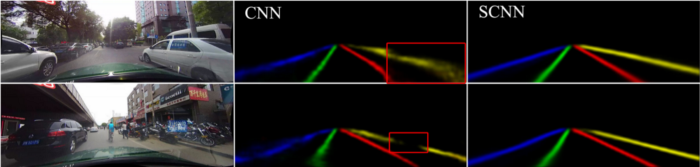
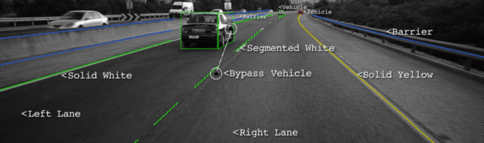
左上方圖像右側(cè)的汽車和左下方圖像右側(cè)的摩托車遮擋了右側(cè)車道標(biāo)記,并對CNN結(jié)果產(chǎn)生負面影響
但是,由于我們知道交通信號桿通常表現(xiàn)出相似的空間關(guān)系,例如垂直站立并放置在道路的左右兩側(cè),因此我們看到了增強空間信息的重要性。接下來是檢測車道的類似情況。
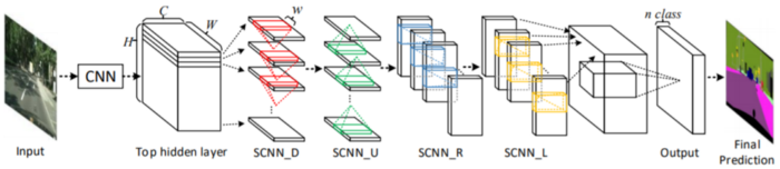
為了解決這個問題,Xingang Pan, Jianping Shi等人提出了一種架構(gòu)Spatial CNN(SCNN),“將傳統(tǒng)的深層逐層卷積概括為特征圖中的逐層卷積”。這是什么意思?在傳統(tǒng)的逐層CNN中,每個卷積層都從其前一層接收輸入,進行卷積和非線性激活,然后將輸出發(fā)送到下一層。SCNN通過將各個要素地圖的行和列視為“層”,進一步采取了這一步驟,并依次應(yīng)用了相同的過程(其中順序表示切片僅在從先前切片接收到信息之后才將信息傳遞給后續(xù)切片),允許像素信息在同一層內(nèi)的神經(jīng)元之間傳遞消息,從而有效地增加了對空間信息的重視。
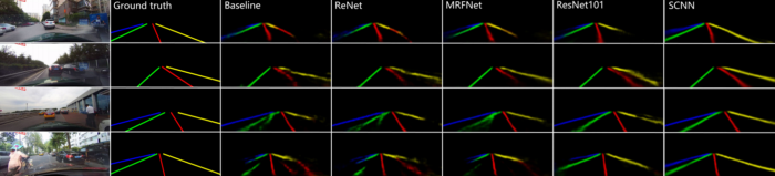
SCNN還相對較新,發(fā)布于2018年,但已經(jīng)跑贏了ReNet(RNN),MRFNet(MRF + CNN),更深入的ResNet架構(gòu)之類,并以96.53% 的準(zhǔn)確性在TuSimple基準(zhǔn)測試車道檢測挑戰(zhàn)賽中排名第一。
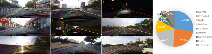
此外,除了SCNN的發(fā)布之外,作者還發(fā)布了CULane Dataset,這是一個大規(guī)模數(shù)據(jù)集,帶有帶有立方棘刺的行車道注釋。CULane數(shù)據(jù)集還包含許多具有挑戰(zhàn)性的場景,包括遮擋和變化的照明條件。
2.模型
車道檢測需要精確的像素識別和車道曲線預(yù)測。SCNN的作者沒有直接訓(xùn)練車道的存在并隨后進行聚類,而是將藍色,綠色,紅色和黃色的車道標(biāo)記視為四個單獨的類。該模型為每個曲線輸出概率圖(概率圖),類似于語義分割任務(wù),然后將概率圖通過一個小型網(wǎng)絡(luò)傳遞,以預(yù)測最終的立方棘。該模型基于DeepLab-LargeFOV模型變體。
GitHub 鏈接 | https://github.com/XingangPan/SCNN
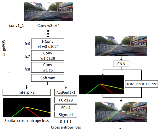
對于存在值超過0.5的每個車道標(biāo)記,將以20行間隔搜索對應(yīng)的概率圖,以找到響應(yīng)度最高的位置。為了確定是否檢測到車道標(biāo)記,計算地面真相(正確標(biāo)簽)和預(yù)測之間的“聯(lián)合路口”(IoU),其中將高于設(shè)置閾值的IoU評估為“真陽性”(TP),以計算精度和記起。
3.測試和訓(xùn)練
全部代碼已經(jīng)上傳至Github上,您可以按照此倉庫在SCNN論文中重現(xiàn)結(jié)果,或使用CULane數(shù)據(jù)集測試您自己的模型。
?? 車道線檢測項目論文和數(shù)據(jù)集 https://github.com/Charmve/Awesome-Lane-Detection
總結(jié)
就是這樣!??希望本教程向您展示了如何使用涉及許多手工功能和微調(diào)的傳統(tǒng)方法來構(gòu)建簡單的車道檢測器,并且還向您介紹了一種替代方法,該方法遵循了解決幾乎所有類型的車輛的最新趨勢。計算機視覺問題:您可以為此添加卷積神經(jīng)網(wǎng)絡(luò)!
更多精彩學(xué)習(xí)資料,承諾大家的,一個也不會少,我分類整理好并附上鏈接。
GitHub上開源:https://github.com/Charmve/computer-vision-in-action
往期精彩回顧
本站qq群851320808,加入微信群請掃碼: