
一行代碼教你繪制頂級期刊要求配圖
↑↑↑關(guān)注后"星標(biāo)"簡說Python 人人都可以簡單入門Python、爬蟲、數(shù)據(jù)分析 簡說Python推薦 來源|python數(shù)據(jù)分析之 作者|小dull鳥
R-ggpubr包主要類型函數(shù)介紹 R-ggpubr包主要案列展示
R-ggpubr包主要類型函數(shù)介紹
雖然在Python中我們也可以通過使用Matplotlib定制化出符合出版要求的圖表,但這畢竟對使用者的繪圖技能要求較高,當(dāng)然也是還有部分輪子可以用的。而我們今天則介紹一個高性能的R包-ggpubr,從名字就可以看出這個包的主要用途了。
官網(wǎng):https://rpkgs.datanovia.com/ggpubr/index.html
幾大繪圖函數(shù)類型
這個包對于繪圖類型分的較為詳細(xì),主要按照變量個數(shù)進(jìn)行劃分,詳細(xì)介紹如下
「繪制一個變量-X,連續(xù)」
ggdensity(): 密度圖 stat_overlay_normal_density(): 覆蓋法線密度圖 gghistogram(): 直方圖 ggecdf(): 經(jīng)驗累積密度函數(shù) ggqqplot(): QQ圖 「繪制兩個變量-X和Y,離散X和連續(xù)Y」
ggboxplot(): 箱形圖 ggviolin(): 小提琴圖 ggdotplot(): 點圖 ggstripchart(): 條形圖 ggbarplot(): 條形圖 ggline(): 線圖 ggerrorplot(): 錯誤圖 ggpie(): 餅圖 ggdonutchart(): 甜甜圈圖 ggdotchart()、theme_cleveland(): 克利夫蘭點圖 ggsummarytable()、ggsummarystats():添加摘要統(tǒng)計信息表 「繪制兩個連續(xù)變量」
ggscatter(): 散點圖 stat_cor(): 將具有P值的相關(guān)系數(shù)添加到散點圖中 stat_stars(): 將星星添加到散點圖中 ggscatterhist(): 具有邊際直方圖的散點圖 「比較均值并添加p值」
compare_means(): 均值比較 stat_compare_means(): 將均值比較P值添加到ggplot stat_pvalue_manual():手動將P值添加到ggplot stat_bracket()、geom_bracket(): 將帶有標(biāo)簽的括號添加到GGPlot
其他更多優(yōu)秀函數(shù),小伙伴們可自行查閱官網(wǎng)進(jìn)行探索。
R-ggpubr包主要案列展示
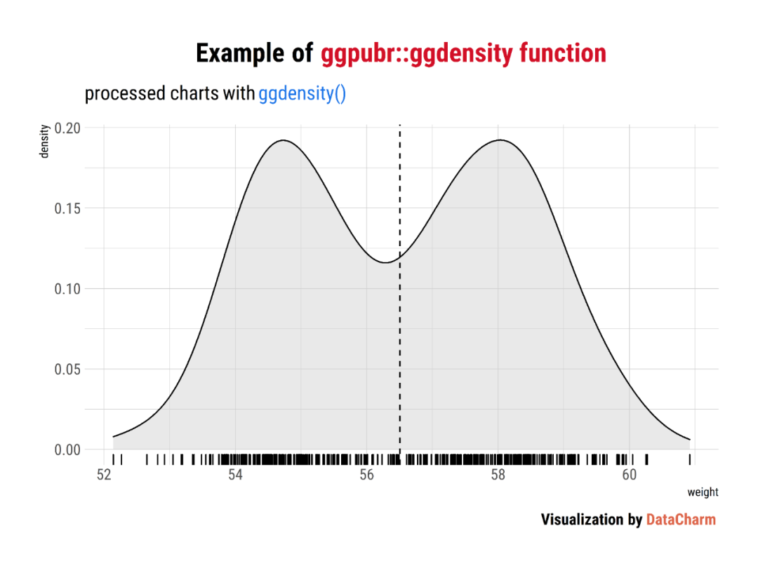
Density plot
set.seed(1234)
wdata = data.frame(
   sex = factor(rep(c("F", "M"), each=200)),
   weight = c(rnorm(200, 55), rnorm(200, 58)))
ggdensity <- ggdensity(wdata, x = "weight", fill = "lightgray",
                       add = "mean", rug = TRUE) +
      labs(
           title = "Example of <span style='color:#D20F26'>ggpubr::ggdensity function</span>",
           subtitle = "processed charts with <span style='color:#1A73E8'>ggdensity()</span>",
           caption = "Visualization by <span style='color:#DD6449'>DataCharm</span>") +
      hrbrthemes::theme_ipsum(base_family = "Roboto Condensed")  +
      theme(
            plot.title = element_markdown(hjust = 0.5,vjust = .5,color = "black",
                                     size = 20, margin = margin(t = 1, b = 12)),
            plot.subtitle = element_markdown(hjust = 0,vjust = .5,size=15),
            plot.caption = element_markdown(face = 'bold',size = 12),
          )
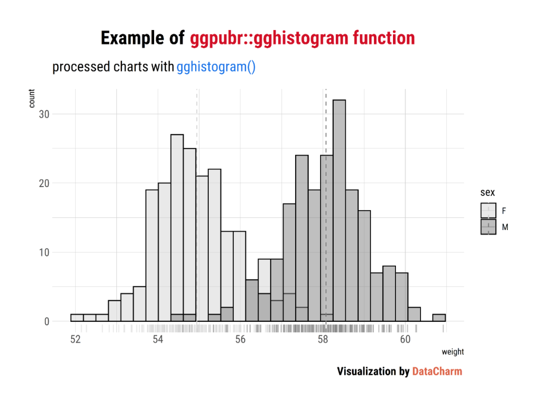
Histogram plot
set.seed(1234)
wdata = data.frame(
   sex = factor(rep(c("F", "M"), each=200)),
   weight = c(rnorm(200, 55), rnorm(200, 58)))

gghistogram <- gghistogram(wdata, x = "weight", fill = "sex",
   add = "mean", palette = c("lightgray", "gray50"),add_density = TRUE,rug = TRUE)+
   labs(
           title = "Example of <span style='color:#D20F26'>ggpubr::gghistogram function</span>",
           subtitle = "processed charts with <span style='color:#1A73E8'>gghistogram()</span>",
           caption = "Visualization by <span style='color:#DD6449'>DataCharm</span>") +
      hrbrthemes::theme_ipsum(base_family = "Roboto Condensed")  +
      theme(
            plot.title = element_markdown(hjust = 0.5,vjust = .5,color = "black",
                                     size = 20, margin = margin(t = 1, b = 12)),
            plot.subtitle = element_markdown(hjust = 0,vjust = .5,size=15),
            plot.caption = element_markdown(face = 'bold',size = 12),
          )
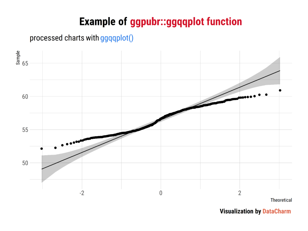
QQ Plots
# Create some data format
set.seed(1234)
wdata = data.frame(
   sex = factor(rep(c("F", "M"), each=200)),
   weight = c(rnorm(200, 55), rnorm(200, 58)))

# Basic QQ plot
ggqqplot <- ggqqplot(wdata, x = "weight") +
   labs(
           title = "Example of <span style='color:#D20F26'>ggpubr::ggqqplot function</span>",
           subtitle = "processed charts with <span style='color:#1A73E8'>ggqqplot()</span>",
           caption = "Visualization by <span style='color:#DD6449'>DataCharm</span>") +
      hrbrthemes::theme_ipsum(base_family = "Roboto Condensed")  +
      theme(
            plot.title = element_markdown(hjust = 0.5,vjust = .5,color = "black",
                                     size = 20, margin = margin(t = 1, b = 12)),
            plot.subtitle = element_markdown(hjust = 0,vjust = .5,size=15),
            plot.caption = element_markdown(face = 'bold',size = 12),
          )
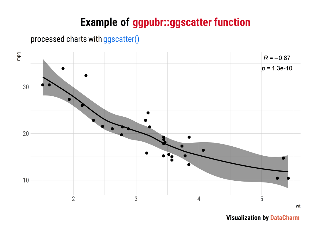
Scatter plot
# Load data
data("mtcars")
df <- mtcars
df$cyl <- as.factor(df$cyl)
ggscatter <- ggscatter(df, x = "wt", y = "mpg",
   add = "loess", conf.int = TRUE,
   cor.coef = TRUE,
   cor.coeff.args = list(method = "pearson", label.x = 5,label.y=35, label.size=25,label.sep = "\n"))+
   labs(
           title = "Example of <span style='color:#D20F26'>ggpubr::ggscatter function</span>",
           subtitle = "processed charts with <span style='color:#1A73E8'>ggscatter()</span>",
           caption = "Visualization by <span style='color:#DD6449'>DataCharm</span>") +
      hrbrthemes::theme_ipsum(base_family = "Roboto Condensed")  +
      theme(
            plot.title = element_markdown(hjust = 0.5,vjust = .5,color = "black",
                                     size = 20, margin = margin(t = 1, b = 12)),
            plot.subtitle = element_markdown(hjust = 0,vjust = .5,size=15),
            plot.caption = element_markdown(face = 'bold',size = 12),
          )
Add Manually P-values to a ggplot
ToothGrowth$dose <- as.factor(ToothGrowth$dose)
# Comparisons against reference
stat.test <- compare_means(
  len ~ dose, data = ToothGrowth, group.by = "supp",
  method = "t.test", ref.group = "0.5"
)

bp <- ggbarplot(ToothGrowth, x = "supp", y = "len",
                fill = "dose", palette = "jco",
                add = "mean_sd", add.params = list(group = "dose"),
                position = position_dodge(0.8))
bp + stat_pvalue_manual(
  stat.test, x = "supp", y.position = 33,
  label = "p.signif",
  position = position_dodge(0.8)
) +
  labs(
           title = "Example of <span style='color:#D20F26'>ggpubr::stat_pvalue_manual function</span>",
           subtitle = "processed charts with <span style='color:#1A73E8'>stat_pvalue_manual()</span>",
           caption = "Visualization by <span style='color:#DD6449'>DataCharm</span>") +
      hrbrthemes::theme_ipsum(base_family = "Roboto Condensed")  +
      theme(
            plot.title = element_markdown(hjust = 0.5,vjust = .5,color = "black",
                                     size = 20, margin = margin(t = 1, b = 12)),
            plot.subtitle = element_markdown(hjust = 0,vjust = .5,size=15),
            plot.caption = element_markdown(face = 'bold',size = 12),
          )

Draw a Textual Table
# data
df <- head(iris)

# Default table
table1 <- ggtexttable(df, rows = NULL)
table2 <- ggtexttable(df, rows = NULL, theme = ttheme("blank")) %>%
 tab_add_hline(at.row = 1:2, row.side = "top", linewidth = 2)
總結(jié)
今天推文我們介紹了「R-ggpubr」實現(xiàn)極少代碼繪制出符合期刊要求的可視化圖表,極大省去了繪制單獨圖表元素的時間,為統(tǒng)計分析及可視化探索提供非常便捷的方式,感興趣的小伙伴可探索更多的繪圖函數(shù)哦~~
掃碼回復(fù):2021
獲取最新學(xué)習(xí)資源

推薦大家關(guān)注兩個公號
分享程序員生活、互聯(lián)網(wǎng)資訊、理財復(fù)盤日記等 專注于Java學(xué)習(xí)分享,從零和你一起學(xué)Java
關(guān)注后回復(fù)【1024】 送上獨家資料 ◆◆◆ 歡迎大家圍觀朋友圈,我的微信:pythonbrief 學(xué)習(xí)更多: 整理了我開始分享學(xué)習(xí)筆記到現(xiàn)在超過250篇優(yōu)質(zhì)文章,涵蓋數(shù)據(jù)分析、爬蟲、機器學(xué)習(xí)等方面,別再說不知道該從哪開始,實戰(zhàn)哪里找了
“點贊”傳統(tǒng)美德不能丟 
掃碼回復(fù):2021
獲取最新學(xué)習(xí)資源
推薦大家關(guān)注兩個公號
學(xué)習(xí)更多: 整理了我開始分享學(xué)習(xí)筆記到現(xiàn)在超過250篇優(yōu)質(zhì)文章,涵蓋數(shù)據(jù)分析、爬蟲、機器學(xué)習(xí)等方面,別再說不知道該從哪開始,實戰(zhàn)哪里找了
“點贊”傳統(tǒng)美德不能丟
評論
圖片
表情