↑ 關(guān)注 + 星標 ，每天學Python新技能
后臺回復【大禮包】送你Python自學大禮包

本文收集整理了公開網(wǎng)絡(luò)上一些常見的異常檢測方法（附資料來源和代碼）。

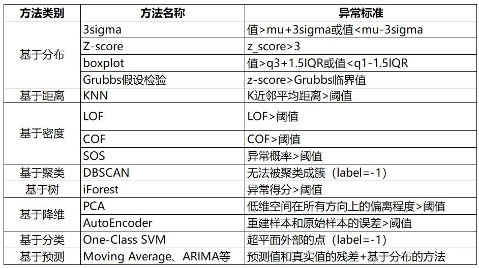
一、基于分布的方法

1. 3sigma

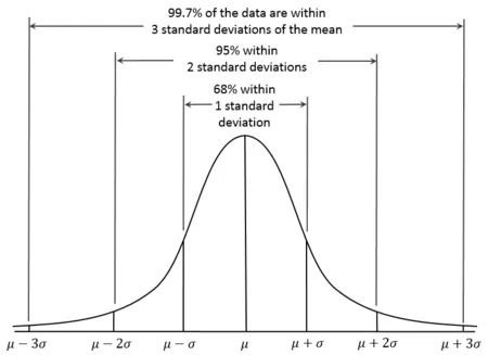
基于正態(tài)分布，3sigma準則認為超過3sigma的數(shù)據(jù)為異常點。

def three_sigma(s):
    mu, std = np.mean(s), np.std(s)
    lower, upper = mu-3*std, mu+3*std
    return lower, upper

2. Z-score

Z-score為標準分數(shù)，測量數(shù)據(jù)點和平均值的距離，若A與平均值相差2個標準差，Z-score為2。當把Z-score=3作為閾值去剔除異常點時，便相當于3sigma。

def z_score(s):
  z_score = (s - np.mean(s)) / np.std(s)
  return z_score

3. boxplot

箱線圖時基于四分位距（IQR）找異常點的。

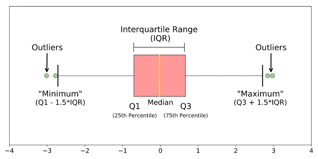
def boxplot(s):
    q1, q3 = s.quantile(.25), s.quantile(.75)
    iqr = q3 - q1
    lower, upper = q1 - 1.5*iqr, q3 + 1.5*iqr
    return lower, upper

4. Grubbs假設(shè)檢驗

資料來源：

[1] 時序預測競賽之異常檢測算法綜述 - 魚遇雨欲語與余，知乎：https://zhuanlan.zhihu.com/p/336944097
[2] 剔除異常值柵格計算器_數(shù)據(jù)分析師所需的統(tǒng)計學：異常檢測 - weixin_39974030，CSDN：https://blog.csdn.net/weixin_39974030/article/details/112569610

Grubbs’Test為一種假設(shè)檢驗的方法，常被用來檢驗服從正態(tài)分布的單變量數(shù)據(jù)集（univariate data set）Y中的單個異常值。若有異常值，則其必為數(shù)據(jù)集中的最大值或最小值。原假設(shè)與備擇假設(shè)如下：

H0: 數(shù)據(jù)集中沒有異常值
H1: 數(shù)據(jù)集中有一個異常值

使用Grubbs測試需要總體是正態(tài)分布的。算法流程：

1. 樣本從小到大排序

2. 求樣本的mean和dev

3. 計算min/max與mean的差距，更大的那個為可疑值

4. 求可疑值的z-score (standard score)，如果大于Grubbs臨界值，那么就是outlier

Grubbs臨界值可以查表得到，它由兩個值決定：檢出水平α（越嚴格越小），樣本數(shù)量n，排除outlier，對剩余序列循環(huán)做 1-4 步驟 [1]。詳細計算樣例可以參考。

from outliers import smirnov_grubbs as grubbs
print(grubbs.test([8, 9, 10, 1, 9], alpha=0.05))
print(grubbs.min_test_outliers([8, 9, 10, 1, 9], alpha=0.05))
print(grubbs.max_test_outliers([8, 9, 10, 1, 9], alpha=0.05))
print(grubbs.max_test_indices([8, 9, 10, 50, 9], alpha=0.05))

局限：

1、只能檢測單維度數(shù)據(jù)

2、無法精確的輸出正常區(qū)間

3、它的判斷機制是“逐一剔除”，所以每個異常值都要單獨計算整個步驟，數(shù)據(jù)量大吃不消。

4、需假定數(shù)據(jù)服從正態(tài)分布或近正態(tài)分布

二、基于距離的方法

1. KNN

資料來源：

[3] 異常檢測算法之(KNN)-K Nearest Neighbors - 小伍哥聊風控，知乎：https://zhuanlan.zhihu.com/p/501691799

依次計算每個樣本點與它最近的K個樣本的平均距離，再利用計算的距離與閾值進行比較，如果大于閾值，則認為是異常點。優(yōu)點是不需要假設(shè)數(shù)據(jù)的分布，缺點是僅可以找出全局異常點，無法找到局部異常點。

from pyod.models.knn import KNN

# 初始化檢測器clf
clf = KNN( method='mean', n_neighbors=3, )
clf.fit(X_train)
# 返回訓練數(shù)據(jù)上的分類標簽 (0: 正常值, 1: 異常值)
y_train_pred = clf.labels_
# 返回訓練數(shù)據(jù)上的異常值 (分值越大越異常)
y_train_scores = clf.decision_scores_

三、基于密度的方法

1. Local Outlier Factor (LOF)

資料來源：

[4] 一文讀懂異常檢測 LOF 算法（Python代碼）- 東哥起飛，知乎：https://zhuanlan.zhihu.com/p/448276009

LOF是基于密度的經(jīng)典算法（Breuning et. al. 2000），通過給每個數(shù)據(jù)點都分配一個依賴于鄰域密度的離群因子 LOF，進而判斷該數(shù)據(jù)點是否為離群點。它的好處在于可以量化每個數(shù)據(jù)點的異常程度（outlierness）。

數(shù)據(jù)點的局部相對密度（局部異常因子）為點鄰域內(nèi)點的平均局部可達密度跟數(shù)據(jù) 點的局部可達密度的比值, 即：

數(shù)據(jù)點P的局部可達密度=P最近鄰的平均可達距離的倒數(shù)。距離越大，密度越小。

點P到點O的第k可達距離=max(點O的k近鄰距離，點P到點O的距離)。

點O的k近鄰距離=第k個最近的點跟點O之間的距離。

整體來說，LOF算法流程如下：

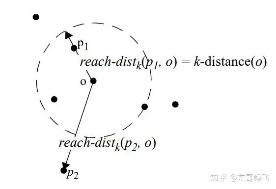
對于每個數(shù)據(jù)點，計算它與其他所有點的距離，并按從近到遠排序；
對于每個數(shù)據(jù)點，找到它的K-Nearest-Neighbor，計算LOF得分。

from sklearn.neighbors import LocalOutlierFactor as LOF

X = [[-1.1], [0.2], [100.1], [0.3]]
clf = LOF(n_neighbors=2)
res = clf.fit_predict(X)
print(res)
print(clf.negative_outlier_factor_)

2. Connectivity-Based Outlier Factor (COF)

資料來源：

[5] Nowak-Brzezińska, A., & Horyń, C. (2020). Outliers in rules-the comparision of LOF, COF and KMEANS algorithms. *Procedia Computer Science*, *176*, 1420-1429.
[6] 機器學習_學習筆記系列(98)：基於連接異常因子分析(Connectivity-Based Outlier Factor) - 劉智皓 (Chih-Hao Liu)

COF是LOF的變種，相比于LOF，COF可以處理低密度下的異常值，COF的局部密度是基于平均鏈式距離計算得到。在一開始的時候我們一樣會先計算出每個點的k-nearest neighbor。而接下來我們會計算每個點的Set based nearest Path，如下圖：

假使我們今天我們的k=5，所以F的neighbor為B、C、D、E、G。而對于F離他最近的點為E，所以SBN Path的第一個元素是F、第二個是E。離E最近的點為D所以第三個元素為D，接下來離D最近的點為C和G，所以第四和五個元素為C和G，最后離C最近的點為B，第六個元素為B。

所以整個流程下來，F(xiàn)的SBN Path為{F, E, D, C, G, C, B}。而對于SBN Path所對應的距離e={e1, e2, e3,…,ek}，依照上面的例子e={3,2,1,1,1}。

所以我們可以說假使我們想計算p點的SBN Path，我們只要直接計算p點和其neighbor所有點所構(gòu)成的graph的minimum spanning tree，之后我們再以p點為起點執(zhí)行shortest path算法，就可以得到我們的SBN Path。

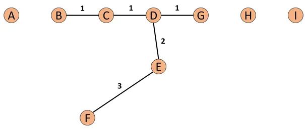
而接下來我們有了SBN Path我們就會接著計算，p點的鏈式距離：

有了ac_distance后，我們就可以計算COF：

# https://zhuanlan.zhihu.com/p/362358580
from pyod.models.cof import COF
cof = COF(contamination = 0.06,  ## 異常值所占的比例
          n_neighbors = 20,      ## 近鄰數(shù)量
        )
cof_label = cof.fit_predict(iris.values) # 鳶尾花數(shù)據(jù)
print("檢測出的異常值數(shù)量為:",np.sum(cof_label == 1))

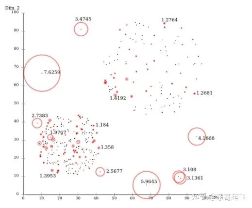
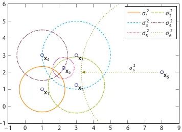
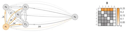
3. Stochastic Outlier Selection (SOS)

資料來源：

[7] 異常檢測之SOS算法 - 呼廣躍，知乎：https://zhuanlan.zhihu.com/p/34438518

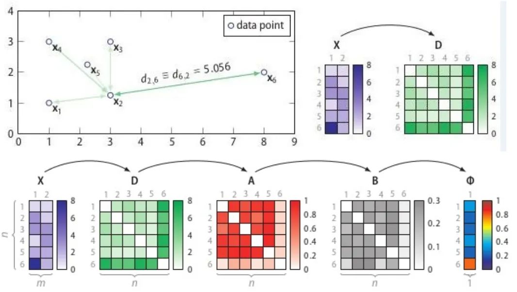
將特征矩陣（feature martrix）或者相異度矩陣（dissimilarity matrix）輸入給SOS算法，會返回一個異常概率值向量（每個點對應一個）。SOS的思想是：當一個點和其它所有點的關(guān)聯(lián)度（affinity）都很小的時候，它就是一個異常點。

SOS的流程：

計算相異度矩陣D；
計算關(guān)聯(lián)度矩陣A；
計算關(guān)聯(lián)概率矩陣B；
算出異常概率向量。

相異度矩陣D是各樣本兩兩之間的度量距離, 比如歐式距離或漢明距離等。關(guān)聯(lián)度矩陣反映的是度量距離方差, 如圖7, 點的密度最大, 方差最小; 的密度最小, 方差最大。而關(guān)聯(lián)概率矩陣 (binding probability matrix)就是把關(guān)聯(lián)矩陣(affinity matrix)按行歸一化得到的, 如圖 8 所示。

得到了binding probability matrix，每個點的異常概率值就用如下的公式計算，當一個點和其它所有點的關(guān)聯(lián)度（affinity）都很小的時候，它就是一個異常點。

# Ref: https://github.com/jeroenjanssens/scikit-sos
import pandas as pd
from sksos import SOS
iris = pd.read_csv("http://bit.ly/iris-csv")
X = iris.drop("Name", axis=1).values
detector = SOS()
iris["score"] = detector.predict(X)
iris.sort_values("score", ascending=False).head(10)

四、基于聚類的方法

1. DBSCAN

DBSCAN算法（Density-Based Spatial Clustering of Applications with Noise）的輸入和輸出如下，對于無法形成聚類簇的孤立點，即為異常點（噪聲點）。

輸入：數(shù)據(jù)集，鄰域半徑Eps，鄰域中數(shù)據(jù)對象數(shù)目閾值MinPts;
輸出：密度聯(lián)通簇。

處理流程如下：

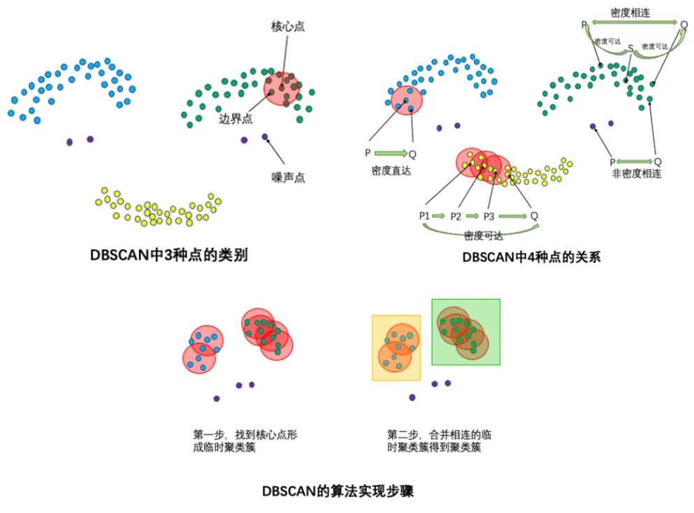
從數(shù)據(jù)集中任意選取一個數(shù)據(jù)對象點p；
如果對于參數(shù)Eps和MinPts，所選取的數(shù)據(jù)對象點p為核心點，則找出所有從p密度可達的數(shù)據(jù)對象點，形成一個簇；
如果選取的數(shù)據(jù)對象點 p 是邊緣點，選取另一個數(shù)據(jù)對象點；
重復以上2、3步，直到所有點被處理。

# Ref: https://zhuanlan.zhihu.com/p/515268801
from sklearn.cluster import DBSCAN
import numpy as np
X = np.array([[1, 2], [2, 2], [2, 3],
              [8, 7], [8, 8], [25, 80]])
clustering = DBSCAN(eps=3, min_samples=2).fit(X)

clustering.labels_
array([ 0,  0,  0,  1,  1, -1])
# 0，,0，,0：表示前三個樣本被分為了一個群
# 1, 1：中間兩個被分為一個群
# -1：最后一個為異常點，不屬于任何一個群

五、基于樹的方法

1. Isolation Forest (iForest)

資料來源：

[8] 異常檢測算法 -- 孤立森林（Isolation Forest）剖析 - 風控大魚，知乎：https://zhuanlan.zhihu.com/p/74508141
[9] 孤立森林(isolation Forest)-一個通過瞎幾把亂分進行異常檢測的算法 - 小伍哥聊風控，知乎：https://zhuanlan.zhihu.com/p/484495545
[10] 孤立森林閱讀 - Mark_Aussie，博文：https://blog.csdn.net/MarkAustralia/article/details/120181899

孤立森林中的 “孤立” (isolation) 指的是 “把異常點從所有樣本中孤立出來”，論文中的原文是 “separating an instance from the rest of the instances”。

我們用一個隨機超平面對一個數(shù)據(jù)空間進行切割，切一次可以生成兩個子空間。接下來，我們再繼續(xù)隨機選取超平面，來切割第一步得到的兩個子空間，以此循環(huán)下去，直到每子空間里面只包含一個數(shù)據(jù)點為止。

我們可以發(fā)現(xiàn)，那些密度很高的簇要被切很多次才會停止切割，即每個點都單獨存在于一個子空間內(nèi)，但那些分布稀疏的點，大都很早就停到一個子空間內(nèi)了。所以，整個孤立森林的算法思想：異常樣本更容易快速落入葉子結(jié)點或者說，異常樣本在決策樹上，距離根節(jié)點更近。

隨機選擇m個特征，通過在所選特征的最大值和最小值之間隨機選擇一個值來分割數(shù)據(jù)點。觀察值的劃分遞歸地重復，直到所有的觀察值被孤立。

獲得 t 個孤立樹后，單棵樹的訓練就結(jié)束了。接下來就可以用生成的孤立樹來評估測試數(shù)據(jù)了，即計算異常分數(shù) s。對于每個樣本 x，需要對其綜合計算每棵樹的結(jié)果，通過下面的公式計算異常得分：

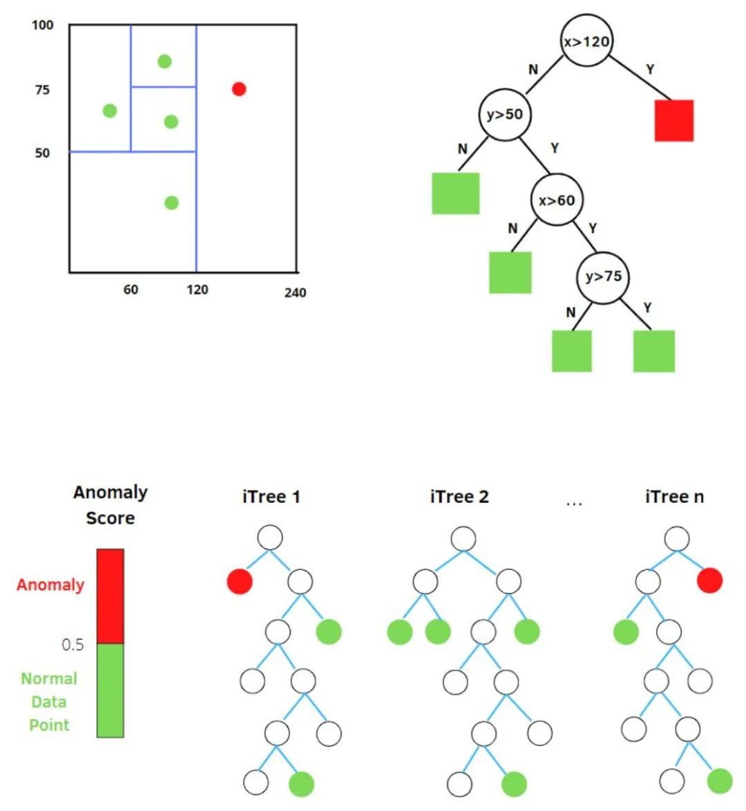
h(x)：為樣本在iTree上的PathLength；
E(h(x))：為樣本在t棵iTree的PathLength的均值；
: 為個樣本構(gòu)建一個二叉搜索樹BST中的末成功搜索平均路徑長度 (均值h(x)對外部節(jié)點終端的估計等同于BST中的末成功搜索）。是對樣本x的路徑長度進行標準化處理。是調(diào)和數(shù), 可使用 (歐拉常數(shù)) 估算。

指數(shù)部分值域為(?∞,0)，因此s值域為(0,1)。當PathLength越小，s越接近1，此時樣本為異常值的概率越大。

# Ref：https://zhuanlan.zhihu.com/p/484495545
from sklearn.datasets import load_iris 
from sklearn.ensemble import IsolationForest

data = load_iris(as_frame=True) 
X,y = data.data,data.target 
df = data.frame 

# 模型訓練
iforest = IsolationForest(n_estimators=100, max_samples='auto',  
                          contamination=0.05, max_features=4,  
                          bootstrap=False, n_jobs=-1, random_state=1)

#  fit_predict 函數(shù) 訓練和預測一起 可以得到模型是否異常的判斷，-1為異常，1為正常
df['label'] = iforest.fit_predict(X) 

# 預測 decision_function 可以得出 異常評分
df['scores'] = iforest.decision_function(X)

六、基于降維的方法

1. Principal Component Analysis (PCA)

資料來源：

[11] 機器學習-異常檢測算法（三）：Principal Component Analysis - 劉騰飛，知乎：https://zhuanlan.zhihu.com/p/29091645
[12] Anomaly Detection異常檢測--PCA算法的實現(xiàn) - CC思SS，知乎：https://zhuanlan.zhihu.com/p/48110105

PCA在異常檢測方面的做法，大體有兩種思路：

(1) 將數(shù)據(jù)映射到低維特征空間，然后在特征空間不同維度上查看每個數(shù)據(jù)點跟其它數(shù)據(jù)的偏差；

(2) 將數(shù)據(jù)映射到低維特征空間，然后由低維特征空間重新映射回原空間，嘗試用低維特征重構(gòu)原始數(shù)據(jù)，看重構(gòu)誤差的大小。

PCA在做特征值分解，會得到：

特征向量：反應了原始數(shù)據(jù)方差變化程度的不同方向；
特征值：數(shù)據(jù)在對應方向上的方差大小。

所以，最大特征值對應的特征向量為數(shù)據(jù)方差最大的方向，最小特征值對應的特征向量為數(shù)據(jù)方差最小的方向。原始數(shù)據(jù)在不同方向上的方差變化反應了其內(nèi)在特點。如果單個數(shù)據(jù)樣本跟整體數(shù)據(jù)樣本表現(xiàn)出的特點不太一致，比如在某些方向上跟其它數(shù)據(jù)樣本偏離較大，可能就表示該數(shù)據(jù)樣本是一個異常點。

在前面提到第一種做法中，樣本的異常分數(shù)為該樣本在所有方向上的偏離程度：

其中, 為樣本在重構(gòu)空間里離特征向量的距離。若存在樣本點偏離各主成分越遠, 會越大, 意味偏移程度大, 異常分數(shù)高。是特征值, 用于歸一化, 使不同方向上的偏離程度具有可比性。

在計算異常分數(shù)時，關(guān)于特征向量（即度量異常用的標桿）選擇又有兩種方式：

考慮在前k個特征向量方向上的偏差：前k個特征向量往往直接對應原始數(shù)據(jù)里的某幾個特征，在前幾個特征向量方向上偏差比較大的數(shù)據(jù)樣本，往往就是在原始數(shù)據(jù)中那幾個特征上的極值點。
考慮后r個特征向量方向上的偏差：后r個特征向量通常表示某幾個原始特征的線性組合，線性組合之后的方差比較小反應了這幾個特征之間的某種關(guān)系。在后幾個特征方向上偏差比較大的數(shù)據(jù)樣本，表示它在原始數(shù)據(jù)里對應的那幾個特征上出現(xiàn)了與預計不太一致的情況。

得分大于閾值C則判斷為異常。

第二種做法，PCA提取了數(shù)據(jù)的主要特征，如果一個數(shù)據(jù)樣本不容易被重構(gòu)出來，表示這個數(shù)據(jù)樣本的特征跟整體數(shù)據(jù)樣本的特征不一致，那么它顯然就是一個異常的樣本：

其中, 是基于維特征向量重構(gòu)的樣本。

基于低維特征進行數(shù)據(jù)樣本的重構(gòu)時，舍棄了較小的特征值對應的特征向量方向上的信息。換一句話說，重構(gòu)誤差其實主要來自較小的特征值對應的特征向量方向上的信息。基于這個直觀的理解，PCA在異常檢測上的兩種不同思路都會特別關(guān)注較小的特征值對應的特征向量。所以，我們說PCA在做異常檢測時候的兩種思路本質(zhì)上是相似的，當然第一種方法還可以關(guān)注較大特征值對應的特征向量。

# Ref: [https://zhuanlan.zhihu.com/p/48110105](https://zhuanlan.zhihu.com/p/48110105)
from sklearn.decomposition import PCA
pca = PCA()
pca.fit(centered_training_data)
transformed_data = pca.transform(training_data)
y = transformed_data

# 計算異常分數(shù)
lambdas = pca.singular_values_
M = ((y*y)/lambdas)

# 前k個特征向量和后r個特征向量
q = 5
print "Explained variance by first q terms: ", sum(pca.explained_variance_ratio_[:q])
q_values = list(pca.singular_values_ < .2)
r = q_values.index(True)

# 對每個樣本點進行距離求和的計算
major_components = M[:,range(q)]
minor_components = M[:,range(r, len(features))]
major_components = np.sum(major_components, axis=1)
minor_components = np.sum(minor_components, axis=1)

# 人為設(shè)定c1、c2閾值
components = pd.DataFrame({'major_components': major_components, 
                               'minor_components': minor_components})
c1 = components.quantile(0.99)['major_components']
c2 = components.quantile(0.99)['minor_components']

# 制作分類器
def classifier(major_components, minor_components):  
    major = major_components > c1
    minor = minor_components > c2    
    return np.logical_or(major,minor)

results = classifier(major_components=major_components, minor_components=minor_components)

2. AutoEncoder

資料來源：

[13] 利用Autoencoder進行無監(jiān)督異常檢測(Python) - SofaSofa.io，知乎：https://zhuanlan.zhihu.com/p/46188296
[14] 自編碼器AutoEncoder解決異常檢測問題（手把手寫代碼） - 數(shù)據(jù)如琥珀，知乎：https://zhuanlan.zhihu.com/p/260882741

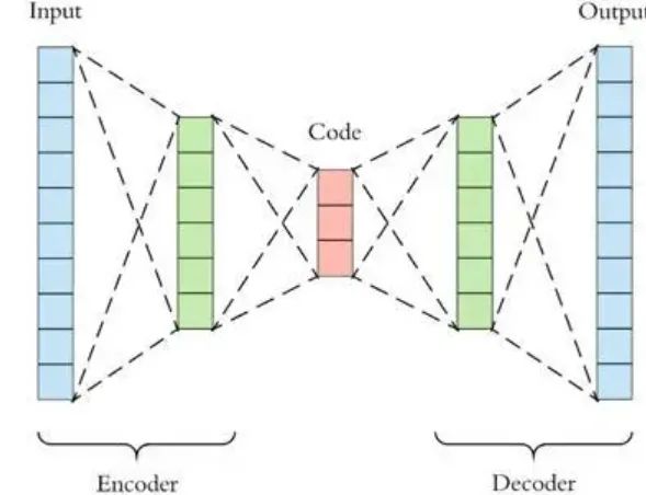
PCA是線性降維，AutoEncoder是非線性降維。根據(jù)正常數(shù)據(jù)訓練出來的AutoEncoder，能夠?qū)⒄颖局亟ㄟ€原，但是卻無法將異于正常分布的數(shù)據(jù)點較好地還原，導致還原誤差較大。因此如果一個新樣本被編碼，解碼之后，它的誤差超出正常數(shù)據(jù)編碼和解碼后的誤差范圍，則視作為異常數(shù)據(jù)。

需要注意的是，AutoEncoder訓練使用的數(shù)據(jù)是正常數(shù)據(jù)（即無異常值），這樣才能得到重構(gòu)后誤差分布范圍是多少以內(nèi)是合理正常的。所以AutoEncoder在這里做異常檢測時，算是一種有監(jiān)督學習的方法。

# Ref: [https://zhuanlan.zhihu.com/p/260882741](https://zhuanlan.zhihu.com/p/260882741)
import tensorflow as tf
from keras.models import Sequential
from keras.layers import Dense

# 標準化數(shù)據(jù)
scaler = preprocessing.MinMaxScaler()
X_train = pd.DataFrame(scaler.fit_transform(dataset_train),
                              columns=dataset_train.columns,
                              index=dataset_train.index)
# Random shuffle training data
X_train.sample(frac=1)
X_test = pd.DataFrame(scaler.transform(dataset_test),
                             columns=dataset_test.columns,
                             index=dataset_test.index)

tf.random.set_seed(10)
act_func = 'relu'
# Input layer:
model=Sequential()
# First hidden layer, connected to input vector X.
model.add(Dense(10,activation=act_func,
                kernel_initializer='glorot_uniform',
                kernel_regularizer=regularizers.l2(0.0),
                input_shape=(X_train.shape[1],)
               )
         )
model.add(Dense(2,activation=act_func,
                kernel_initializer='glorot_uniform'))
model.add(Dense(10,activation=act_func,
                kernel_initializer='glorot_uniform'))
model.add(Dense(X_train.shape[1],
                kernel_initializer='glorot_uniform'))
model.compile(loss='mse',optimizer='adam')
print(model.summary())

# Train model for 100 epochs, batch size of 10:
NUM_EPOCHS=100
BATCH_SIZE=10
history=model.fit(np.array(X_train),np.array(X_train),
                  batch_size=BATCH_SIZE,
                  epochs=NUM_EPOCHS,
                  validation_split=0.05,
                  verbose = 1)

plt.plot(history.history['loss'],
         'b',
         label='Training loss')
plt.plot(history.history['val_loss'],
         'r',
         label='Validation loss')
plt.legend(loc='upper right')
plt.xlabel('Epochs')
plt.ylabel('Loss, [mse]')
plt.ylim([0,.1])
plt.show()

# 查看訓練集還原的誤差分布如何，以便制定正常的誤差分布范圍
X_pred = model.predict(np.array(X_train))
X_pred = pd.DataFrame(X_pred,
                      columns=X_train.columns)
X_pred.index = X_train.index

scored = pd.DataFrame(index=X_train.index)
scored['Loss_mae'] = np.mean(np.abs(X_pred-X_train), axis = 1)
plt.figure()
sns.distplot(scored['Loss_mae'],
             bins = 10,
             kde= True,
            color = 'blue')
plt.xlim([0.0,.5])

# 誤差閾值比對，找出異常值
X_pred = model.predict(np.array(X_test))
X_pred = pd.DataFrame(X_pred,
                      columns=X_test.columns)
X_pred.index = X_test.index
threshod = 0.3
scored = pd.DataFrame(index=X_test.index)
scored['Loss_mae'] = np.mean(np.abs(X_pred-X_test), axis = 1)
scored['Threshold'] = threshod
scored['Anomaly'] = scored['Loss_mae'] > scored['Threshold']
scored.head()

七、基于分類的方法

1. One-Class SVM

資料來源：

[15] Python機器學習筆記：One Class SVM - zoukankan，博文：http://t.zoukankan.com/wj-1314-p-10701708.html
[16] 單類SVM: SVDD - 張義策，知乎：https://zhuanlan.zhihu.com/p/65617987

One-Class SVM，這個算法的思路非常簡單，就是尋找一個超平面將樣本中的正例圈出來，預測就是用這個超平面做決策，在圈內(nèi)的樣本就認為是正樣本，在圈外的樣本是負樣本，用在異常檢測中，負樣本可看作異常樣本。它屬于無監(jiān)督學習，所以不需要標簽。

One-Class SVM又一種推導方式是SVDD（Support Vector Domain Description，支持向量域描述），對于SVDD來說，我們期望所有不是異常的樣本都是正類別，同時它采用一個超球體，而不是一個超平面來做劃分，該算法在特征空間中獲得數(shù)據(jù)周圍的球形邊界，期望最小化這個超球體的體積，從而最小化異常點數(shù)據(jù)的影響。

假設(shè)產(chǎn)生的超球體參數(shù)為中心 o 和對應的超球體半徑r>0，超球體體積V(r)被最小化，中心o是支持行了的線性組合；跟傳統(tǒng)SVM方法相似，可以要求所有訓練數(shù)據(jù)點xi到中心的距離嚴格小于r。但是同時構(gòu)造一個懲罰系數(shù)為C的松弛變量 ζi，優(yōu)化問題入下所示：

C是調(diào)節(jié)松弛變量的影響大小，說的通俗一點就是，給那些需要松弛的數(shù)據(jù)點多少松弛空間，如果C比較小，會給離群點較大的彈性，使得它們可以不被包含進超球體。詳細推導過程參考資料[15] [16]。

from sklearn import svm
# fit the model
clf = svm.OneClassSVM(nu=0.1, kernel='rbf', gamma=0.1)
clf.fit(X)
y_pred = clf.predict(X)
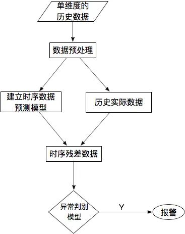
n_error_outlier = y_pred[y_pred == -1].size

八、基于預測的方法

資料來源：

[17] 【TS技術(shù)課堂】時間序列異常檢測 - 時序人，文章：https://mp.weixin.qq.com/s/9TimTB_ccPsme2MNPuy6uA

對于單條時序數(shù)據(jù)，根據(jù)其預測出來的時序曲線和真實的數(shù)據(jù)相比，求出每個點的殘差，并對殘差序列建模，利用KSigma或者分位數(shù)等方法便可以進行異常檢測。具體的流程如下：

九、總結(jié)

異常檢測方法總結(jié)如下：

參考資料

[1] 時序預測競賽之異常檢測算法綜述

- 魚遇雨欲語與余，知乎：

https://zhuanlan.zhihu.com/p/336944097

[2] 剔除異常值柵格計算器_數(shù)據(jù)分析師所需的統(tǒng)計學：

異常檢測 - weixin_39974030，CSDN：

https://blog.csdn.net/weixin_39974030/article/details/112569610

[3] 異常檢測算法之(KNN)-K Nearest Neighbors

- 小伍哥聊風控，知乎：

https://zhuanlan.zhihu.com/p/501691799

[4] 一文讀懂異常檢測 LOF 算法（Python代碼）

- 東哥起飛，知乎：

https://zhuanlan.zhihu.com/p/448276009

[5] Nowak-Brzezińska, A., & Horyń, C. (2020). Outliers in rules-the comparision of LOF, COF and KMEANS algorithms.

*Procedia Computer Science*, *176*, 1420-1429.

[6] 機器學習_學習筆記系列(98)：

基於連接異常因子分析(Connectivity-Based Outlier Factor)

- 劉智皓 (Chih-Hao Liu)

[7] 異常檢測之SOS算法 - 呼廣躍，知乎：

https://zhuanlan.zhihu.com/p/34438518

[8] 異常檢測算法 -- 孤立森林（Isolation Forest）剖析

- 風控大魚，知乎：

https://zhuanlan.zhihu.com/p/74508141

[9] 孤立森林(isolation Forest)-一個通過瞎幾把亂分進行異常檢測的算法

- 小伍哥聊風控，知乎：

https://zhuanlan.zhihu.com/p/484495545

[10] 孤立森林閱讀 - Mark_Aussie，博文：

https://blog.csdn.net/MarkAustralia/article/details/12018189

[11] 機器學習-異常檢測算法（三）：

Principal Component Analysis - 劉騰飛，知乎：

https://zhuanlan.zhihu.com/p/29091645

[12] Anomaly Detection異常檢測--PCA算法的實現(xiàn)

- CC思SS，知乎：

https://zhuanlan.zhihu.com/p/48110105

[13] 利用Autoencoder進行無監(jiān)督異常檢測(Python)

- SofaSofa.io，知乎：

https://zhuanlan.zhihu.com/p/46188296

[14] 自編碼器AutoEncoder解決異常檢測問題

（手把手寫代碼） - 數(shù)據(jù)如琥珀，知乎：

https://zhuanlan.zhihu.com/p/260882741

[15] Python機器學習筆記：

One Class SVM - zoukankan，博文：

http://t.zoukankan.com/wj-1314-p-10701708.html

[16] 單類SVM: SVDD - 張義策，知乎：

https://zhuanlan.zhihu.com/p/65617987[17]

[17]【TS技術(shù)課堂】時間序列異常檢測 - 時序人，文章：

https://mp.weixin.qq.com/s/9TimTB_ccPsme2MNPuy6uA

向下滑動查看

來源：宅碼

細思恐極，插上 U 盤就開始執(zhí)行 Python 代碼
不要再寫Python for循環(huán)了
推薦 GitHub 上的一套公開 API 接口，簡直不要太全！

收藏！14 種異常檢測方法總結(jié)

↑ 關(guān)注 + 星標，每天學Python新技能

后臺回復【大禮包】送你Python自學大禮包

一、基于分布的方法

1. 3sigma

2. Z-score

3. boxplot

4. Grubbs假設(shè)檢驗

二、基于距離的方法

1. KNN

三、基于密度的方法

1. Local Outlier Factor (LOF)

2. Connectivity-Based Outlier Factor (COF)

3. Stochastic Outlier Selection (SOS)

四、基于聚類的方法

1. DBSCAN

五、基于樹的方法

1. Isolation Forest (iForest)

六、基于降維的方法

1. Principal Component Analysis (PCA)

2. AutoEncoder

七、基于分類的方法

1. One-Class SVM

八、基于預測的方法

九、總結(jié)

收藏！14 種異常檢測方法總結(jié)

↑ 關(guān)注 + 星標 ，每天學Python新技能

后臺回復【大禮包】送你Python自學大禮包

一、基于分布的方法

1. 3sigma

2. Z-score

3. boxplot

4. Grubbs假設(shè)檢驗

二、基于距離的方法

1. KNN

三、基于密度的方法

1. Local Outlier Factor (LOF)

2. Connectivity-Based Outlier Factor (COF)

3. Stochastic Outlier Selection (SOS)

四、基于聚類的方法

1. DBSCAN

五、基于樹的方法

1. Isolation Forest (iForest)

六、基于降維的方法

1. Principal Component Analysis (PCA)

2. AutoEncoder

七、基于分類的方法

1. One-Class SVM

八、基于預測的方法

九、總結(jié)

↑ 關(guān)注 + 星標，每天學Python新技能