萬字長文總結(jié)機器學(xué)習(xí)的模型評估與調(diào)參
機器學(xué)習(xí)
Author:Samshare
From:SAMshare
? ? ?

選自?Python-Machine-Learning-Book On GitHub
作者:Sebastian Raschka
翻譯&整理 By Sam
由于文章較長,所以我還是先把目錄提前。
?????
一、認識管道流
????1.1 數(shù)據(jù)導(dǎo)入
????1.2 使用管道創(chuàng)建工作流
二、K折交叉驗證
??? 2.1 K折交叉驗證原理
??? 2.2 K折交叉驗證實現(xiàn)
三、曲線調(diào)參
????3.1 模型準(zhǔn)確度
????3.2?繪制學(xué)習(xí)曲線得到樣本數(shù)與準(zhǔn)確率的關(guān)系
????3.3?繪制驗證曲線得到超參和準(zhǔn)確率關(guān)系
四、網(wǎng)格搜索
????4.1?兩層for循環(huán)暴力檢索
????4.2?構(gòu)建字典暴力檢索
五、嵌套交叉驗證
六、相關(guān)評價指標(biāo)
????6.1 混淆矩陣及其實現(xiàn)
????6.2 相關(guān)評價指標(biāo)實現(xiàn)
????6.3 ROC曲線及其實現(xiàn)
一、認識管道流 ?
今天先介紹一下管道工作流的操作。
“管道工作流”這個概念可能有點陌生,其實可以理解為一個容器,然后把我們需要進行的操作都封裝在這個管道里面進行操作,比如數(shù)據(jù)標(biāo)準(zhǔn)化、特征降維、主成分分析、模型預(yù)測等等,下面還是以一個實例來講解。
1.1 數(shù)據(jù)導(dǎo)入與預(yù)處理
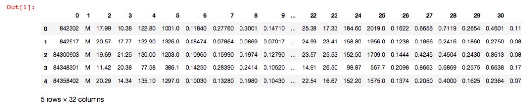
本次我們導(dǎo)入一個二分類數(shù)據(jù)集 Breast Cancer Wisconsin,它包含569個樣本。首列為主鍵ID,第2列為類別值(M=惡性腫瘤,B=良性腫瘤),第3-32列是實數(shù)值的特征。
先導(dǎo)入數(shù)據(jù)集:
 1#?導(dǎo)入相關(guān)數(shù)據(jù)集
 2import?pandas?as?pd
 3import?urllib
 4try:
 5????df?=?pd.read_csv('https://archive.ics.uci.edu/ml/machine-learning-databases'
 6?????????????????????'/breast-cancer-wisconsin/wdbc.data',?header=None)
 7except?urllib.error.URLError:
 8????df?=?pd.read_csv('https://raw.githubusercontent.com/rasbt/'
 9?????????????????????'python-machine-learning-book/master/code/'
10?????????????????????'datasets/wdbc/wdbc.data',?header=None)
11print('rows,?columns:',?df.shape)
12df.head()
使用我們學(xué)習(xí)過的LabelEncoder來轉(zhuǎn)化類別特征:
1from?sklearn.preprocessing?import?LabelEncoder
2X?=?df.loc[:,?2:].values
3y?=?df.loc[:,?1].values
4le?=?LabelEncoder()
5#?將目標(biāo)轉(zhuǎn)為0-1變量
6y?=?le.fit_transform(y)
7le.transform(['M',?'B'])
劃分訓(xùn)練驗證集:
1##?創(chuàng)建訓(xùn)練集和測試集
2from?sklearn.model_selection?import?train_test_split
3X_train,?X_test,?y_train,?y_test?=?\
4????train_test_split(X,?y,?test_size=0.20,?random_state=1)
1.2 使用管道創(chuàng)建工作流
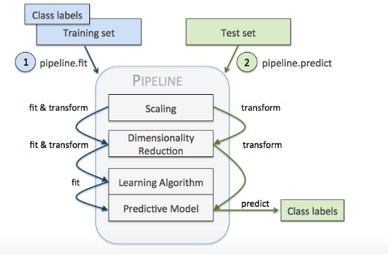
很多機器學(xué)習(xí)算法要求特征取值范圍要相同,因此需要對特征做標(biāo)準(zhǔn)化處理。此外,我們還想將原始的30維度特征壓縮至更少維度,這就需要用到主成分分析,要用PCA來完成,再接著就可以進行l(wèi)ogistic回歸預(yù)測了。
Pipeline對象接收元組構(gòu)成的列表作為輸入,每個元組第一個值作為變量名,元組第二個元素是sklearn中的transformer或Estimator。管道中間每一步由sklearn中的transformer構(gòu)成,最后一步是一個Estimator。
本次數(shù)據(jù)集中,管道包含兩個中間步驟:StandardScaler和PCA,其都屬于transformer,而邏輯斯蒂回歸分類器屬于Estimator。
本次實例,當(dāng)管道pipe_lr執(zhí)行fit方法時:
1)StandardScaler執(zhí)行fit和transform方法;
2)將轉(zhuǎn)換后的數(shù)據(jù)輸入給PCA;
3)PCA同樣執(zhí)行fit和transform方法;
4)最后數(shù)據(jù)輸入給LogisticRegression,訓(xùn)練一個LR模型。
對于管道來說,中間有多少個transformer都可以。管道的工作方式可以用下圖來展示(一定要注意管道執(zhí)行fit方法,而transformer要執(zhí)行fit_transform):
上面的代碼實現(xiàn)如下:
 1from?sklearn.preprocessing?import?StandardScaler?#?用于進行數(shù)據(jù)標(biāo)準(zhǔn)化
 2from?sklearn.decomposition?import?PCA?#?用于進行特征降維
 3from?sklearn.linear_model?import?LogisticRegression?#?用于模型預(yù)測
 4from?sklearn.pipeline?import?Pipeline
 5pipe_lr?=?Pipeline([('scl',?StandardScaler()),
 6????????????????????('pca',?PCA(n_components=2)),
 7????????????????????('clf',?LogisticRegression(random_state=1))])
 8pipe_lr.fit(X_train,?y_train)
 9print('Test?Accuracy:?%.3f'?%?pipe_lr.score(X_test,?y_test))
10y_pred?=?pipe_lr.predict(X_test)
Test Accuracy: 0.947
二、K折交叉驗證 ?
為什么要評估模型的泛化能力,相信這個大家應(yīng)該沒有疑惑,一個模型如果性能不好,要么是因為模型過于復(fù)雜導(dǎo)致過擬合(高方差),要么是模型過于簡單導(dǎo)致導(dǎo)致欠擬合(高偏差)。如何評估它,用什么數(shù)據(jù)來評估它,成為了模型評估需要重點考慮的問題。
我們常規(guī)做法,就是將數(shù)據(jù)集劃分為3部分,分別是訓(xùn)練、測試和驗證,彼此之間的數(shù)據(jù)不重疊。但,如果我們遇見了數(shù)據(jù)量不多的時候,這種操作就顯得不太現(xiàn)實,這個時候k折交叉驗證就發(fā)揮優(yōu)勢了。
2.1 K折交叉驗證原理
先不多說,先貼一張原理圖(以10折交叉驗證為例)。
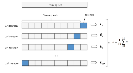
k折交叉驗證步驟:
Step 1:使用不重復(fù)抽樣將原始數(shù)據(jù)隨機分為k份;
Step?2:其中k-1份數(shù)據(jù)用于模型訓(xùn)練,剩下的那1份數(shù)據(jù)用于測試模型;
Step 3:重復(fù)Step 2?k次,得到k個模型和他的評估結(jié)果。
Step 4:計算k折交叉驗證結(jié)果的平均值作為參數(shù)/模型的性能評估。
2.1 K折交叉驗證實現(xiàn)
K折交叉驗證,那么K的取值該如何確認呢?一般我們默認10折,但根據(jù)實際情況有所調(diào)整。我們要知道,當(dāng)K很大的時候,你需要訓(xùn)練的模型就會很多,這樣子對效率影響較大,而且每個模型的訓(xùn)練集都差不多,效果也差不多。我們常用的K值在5~12。
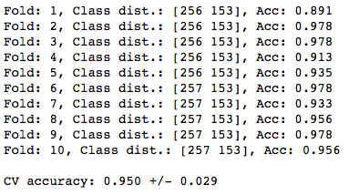
我們根據(jù)k折交叉驗證的原理步驟,在sklearn中進行10折交叉驗證的代碼實現(xiàn):
 1import?numpy?as?np
 2from?sklearn.model_selection?import?StratifiedKFold
 3kfold?=?StratifiedKFold(n_splits=10,
 4????????????????????????????random_state=1).split(X_train,?y_train)
 5scores?=?[]
 6for?k,?(train,?test)?in?enumerate(kfold):
 7????pipe_lr.fit(X_train[train],?y_train[train])
 8????score?=?pipe_lr.score(X_train[test],?y_train[test])
 9????scores.append(score)
10????print('Fold:?%s,?Class?dist.:?%s,?Acc:?%.3f'?%?(k+1,
11??????????np.bincount(y_train[train]),?score))
12print('\nCV?accuracy:?%.3f?+/-?%.3f'?%?(np.mean(scores),?np.std(scores)))
output:
當(dāng)然,實際使用的時候沒必要這樣子寫,sklearn已經(jīng)有現(xiàn)成封裝好的方法,直接調(diào)用即可。
1from?sklearn.model_selection?import?cross_val_score
2scores?=?cross_val_score(estimator=pipe_lr,
3?????????????????????????X=X_train,
4?????????????????????????y=y_train,
5?????????????????????????cv=10,
6?????????????????????????n_jobs=1)
7print('CV?accuracy?scores:?%s'?%?scores)
8print('CV?accuracy:?%.3f?+/-?%.3f'?%?(np.mean(scores),?np.std(scores)))
三、曲線調(diào)參 ?
我們講到的曲線,具體指的是學(xué)習(xí)曲線(learning curve)和驗證曲線(validation curve)。
3.1 模型準(zhǔn)確率(Accuracy)
模型準(zhǔn)確率反饋了模型的效果,大家看下圖:
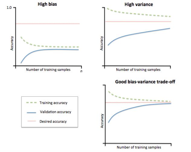
1)左上角子的模型偏差很高。它的訓(xùn)練集和驗證集準(zhǔn)確率都很低,很可能是欠擬合。解決欠擬合的方法就是增加模型參數(shù),比如,構(gòu)建更多的特征,減小正則項。
2)右上角子的模型方差很高,表現(xiàn)就是訓(xùn)練集和驗證集準(zhǔn)確率相差太多。解決過擬合的方法有增大訓(xùn)練集或者降低模型復(fù)雜度,比如增大正則項,或者通過特征選擇減少特征數(shù)。
3)右下角的模型就很好。
3.2 繪制學(xué)習(xí)曲線得到樣本數(shù)與準(zhǔn)確率的關(guān)系
直接上代碼:
 1import?matplotlib.pyplot?as?plt
 2from?sklearn.model_selection?import?learning_curve
 3pipe_lr?=?Pipeline([('scl',?StandardScaler()),
 4????????????????????('clf',?LogisticRegression(penalty='l2',?random_state=0))])
 5train_sizes,?train_scores,?test_scores?=\
 6????????????????learning_curve(estimator=pipe_lr,
 7???????????????????????????????X=X_train,
 8???????????????????????????????y=y_train,
 9???????????????????????????????train_sizes=np.linspace(0.1,?1.0,?10),?#在0.1和1間線性的取10個值
10???????????????????????????????cv=10,
11???????????????????????????????n_jobs=1)
12train_mean?=?np.mean(train_scores,?axis=1)
13train_std?=?np.std(train_scores,?axis=1)
14test_mean?=?np.mean(test_scores,?axis=1)
15test_std?=?np.std(test_scores,?axis=1)
16plt.plot(train_sizes,?train_mean,
17?????????color='blue',?marker='o',
18?????????markersize=5,?label='training?accuracy')
19plt.fill_between(train_sizes,
20?????????????????train_mean?+?train_std,
21?????????????????train_mean?-?train_std,
22?????????????????alpha=0.15,?color='blue')
23plt.plot(train_sizes,?test_mean,
24?????????color='green',?linestyle='--',
25?????????marker='s',?markersize=5,
26?????????label='validation?accuracy')
27plt.fill_between(train_sizes,
28?????????????????test_mean?+?test_std,
29?????????????????test_mean?-?test_std,
30?????????????????alpha=0.15,?color='green')
31plt.grid()
32plt.xlabel('Number?of?training?samples')
33plt.ylabel('Accuracy')
34plt.legend(loc='lower?right')
35plt.ylim([0.8,?1.0])
36plt.tight_layout()
37plt.show()
Learning_curve中的train_sizes參數(shù)控制產(chǎn)生學(xué)習(xí)曲線的訓(xùn)練樣本的絕對/相對數(shù)量,此處,我們設(shè)置的train_sizes=np.linspace(0.1, 1.0, 10),將訓(xùn)練集大小劃分為10個相等的區(qū)間,在0.1和1之間線性的取10個值。learning_curve默認使用分層k折交叉驗證計算交叉驗證的準(zhǔn)確率,我們通過cv設(shè)置k。
下圖可以看到,模型在測試集表現(xiàn)很好,不過訓(xùn)練集和測試集的準(zhǔn)確率還是有一段小間隔,可能是模型有點過擬合。

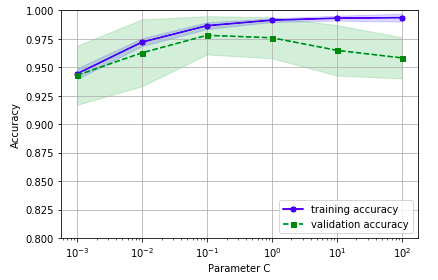
3.3 繪制驗證曲線得到超參和準(zhǔn)確率關(guān)系
驗證曲線是用來提高模型的性能,驗證曲線和學(xué)習(xí)曲線很相近,不同的是這里畫出的是不同參數(shù)下模型的準(zhǔn)確率而不是不同訓(xùn)練集大小下的準(zhǔn)確率:
 1from?sklearn.model_selection?import?validation_curve
 2param_range?=?[0.001,?0.01,?0.1,?1.0,?10.0,?100.0]
 3train_scores,?test_scores?=?validation_curve(
 4????????????????estimator=pipe_lr,?
 5????????????????X=X_train,?
 6????????????????y=y_train,?
 7????????????????param_name='clf__C',?
 8????????????????param_range=param_range,
 9????????????????cv=10)
10train_mean?=?np.mean(train_scores,?axis=1)
11train_std?=?np.std(train_scores,?axis=1)
12test_mean?=?np.mean(test_scores,?axis=1)
13test_std?=?np.std(test_scores,?axis=1)
14plt.plot(param_range,?train_mean,?
15?????????color='blue',?marker='o',?
16?????????markersize=5,?label='training?accuracy')
17plt.fill_between(param_range,?train_mean?+?train_std,
18?????????????????train_mean?-?train_std,?alpha=0.15,
19?????????????????color='blue')
20plt.plot(param_range,?test_mean,?
21?????????color='green',?linestyle='--',?
22?????????marker='s',?markersize=5,?
23?????????label='validation?accuracy')
24plt.fill_between(param_range,?
25?????????????????test_mean?+?test_std,
26?????????????????test_mean?-?test_std,?
27?????????????????alpha=0.15,?color='green')
28plt.grid()
29plt.xscale('log')
30plt.legend(loc='lower?right')
31plt.xlabel('Parameter?C')
32plt.ylabel('Accuracy')
33plt.ylim([0.8,?1.0])
34plt.tight_layout()
35plt.show()
我們得到了參數(shù)C的驗證曲線。和learning_curve方法很像,validation_curve方法使用采樣k折交叉驗證來評估模型的性能。在validation_curve內(nèi)部,我們設(shè)定了用來評估的參數(shù)(這里我們設(shè)置C作為觀測)。
從下圖可以看出,最好的C值是0.1。
四、網(wǎng)格搜索
網(wǎng)格搜索(grid search),作為調(diào)參很常用的方法,這邊還是要簡單介紹一下。
在我們的機器學(xué)習(xí)算法中,有一類參數(shù),需要人工進行設(shè)定,我們稱之為“超參”,也就是算法中的參數(shù),比如學(xué)習(xí)率、正則項系數(shù)或者決策樹的深度等。
網(wǎng)格搜索就是要找到一個最優(yōu)的參數(shù),從而使得模型的效果最佳,而它實現(xiàn)的原理其實就是暴力搜索;即我們事先為每個參數(shù)設(shè)定一組值,然后窮舉各種參數(shù)組合,找到最好的那一組。
4.1. 兩層for循環(huán)暴力檢索
網(wǎng)格搜索的結(jié)果獲得了指定的最優(yōu)參數(shù)值,c為100,gamma為0.001
 1#?naive?grid?search?implementation
 2from?sklearn.datasets?import?load_iris
 3from?sklearn.svm?import?SVC
 4from?sklearn.model_selection?import?train_test_split
 5iris?=?load_iris()
 6X_train,?X_test,?y_train,?y_test?=?train_test_split(iris.data,?iris.target,?random_state=0)
 7print("Size?of?training?set:?%d???size?of?test?set:?%d"?%?(X_train.shape[0],?X_test.shape[0]))
 8best_score?=?0
 9for?gamma?in?[0.001,?0.01,?0.1,?1,?10,?100]:
10????for?C?in?[0.001,?0.01,?0.1,?1,?10,?100]:
11????????#?for?each?combination?of?parameters
12????????#?train?an?SVC
13????????svm?=?SVC(gamma=gamma,?C=C)
14????????svm.fit(X_train,?y_train)
15????????#?evaluate?the?SVC?on?the?test?set?
16????????score?=?svm.score(X_test,?y_test)
17????????#?if?we?got?a?better?score,?store?the?score?and?parameters
18????????if?score?>?best_score:
19????????????best_score?=?score
20????????????best_parameters?=?{'C':?C,?'gamma':?gamma}
21print("best?score:?",?best_score)
22print("best?parameters:?",?best_parameters)
output:
Size of training set: 112 size of test set: 38
best score: 0.973684210526
best parameters: {'C': 100, 'gamma': 0.001}
4.2. 構(gòu)建字典暴力檢索
網(wǎng)格搜索的結(jié)果獲得了指定的最優(yōu)參數(shù)值,c為1
 1from?sklearn.svm?import?SVC
 2from?sklearn.model_selection?import?GridSearchCV
 3pipe_svc?=?Pipeline([('scl',?StandardScaler()),
 4????????????('clf',?SVC(random_state=1))])
 5param_range?=?[0.0001,?0.001,?0.01,?0.1,?1.0,?10.0,?100.0,?1000.0]
 6param_grid?=?[{'clf__C':?param_range,?
 7???????????????'clf__kernel':?['linear']},
 8?????????????????{'clf__C':?param_range,?
 9??????????????????'clf__gamma':?param_range,?
10??????????????????'clf__kernel':?['rbf']}]
11gs?=?GridSearchCV(estimator=pipe_svc,?
12??????????????????param_grid=param_grid,?
13??????????????????scoring='accuracy',?
14??????????????????cv=10,
15??????????????????n_jobs=-1)
16gs?=?gs.fit(X_train,?y_train)
17print(gs.best_score_)
18print(gs.best_params_)
output:
0.978021978022
{'clf__C': 0.1, 'clf__kernel': 'linear'}
GridSearchCV中param_grid參數(shù)是字典構(gòu)成的列表。對于線性SVM,我們只評估參數(shù)C;對于RBF核SVM,我們評估C和gamma。最后, 我們通過best_parmas_得到最優(yōu)參數(shù)組合。
接著,我們直接利用最優(yōu)參數(shù)建模(best_estimator_):
1clf?=?gs.best_estimator_
2clf.fit(X_train,?y_train)
3print('Test?accuracy:?%.3f'?%?clf.score(X_test,?y_test))
網(wǎng)格搜索雖然不錯,但是窮舉過于耗時,sklearn中還實現(xiàn)了隨機搜索,使用 RandomizedSearchCV類,隨機采樣出不同的參數(shù)組合。
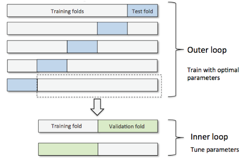
五、嵌套交叉驗證 ?
嵌套交叉驗證(nested cross validation)選擇算法(外循環(huán)通過k折等進行參數(shù)優(yōu)化,內(nèi)循環(huán)使用交叉驗證),對特定數(shù)據(jù)集進行模型選擇。Varma和Simon在論文Bias in Error Estimation When Using Cross-validation for Model Selection中指出使用嵌套交叉驗證得到的測試集誤差幾乎就是真實誤差。
嵌套交叉驗證外部有一個k折交叉驗證將數(shù)據(jù)分為訓(xùn)練集和測試集,內(nèi)部交叉驗證用于選擇模型算法。
下圖演示了一個5折外層交叉沿則和2折內(nèi)部交叉驗證組成的嵌套交叉驗證,也被稱為5*2交叉驗證:
我們還是用到之前的數(shù)據(jù)集,相關(guān)包的導(dǎo)入操作這里就省略了。
SVM分類器的預(yù)測準(zhǔn)確率代碼實現(xiàn):
 1gs?=?GridSearchCV(estimator=pipe_svc,
 2??????????????????param_grid=param_grid,
 3??????????????????scoring='accuracy',
 4??????????????????cv=2)
 5
 6#?Note:?Optionally,?you?could?use?cv=2?
 7#?in?the?GridSearchCV?above?to?produce
 8#?the?5?x?2?nested?CV?that?is?shown?in?the?figure.
 9
10scores?=?cross_val_score(gs,?X_train,?y_train,?scoring='accuracy',?cv=5)
11print('CV?accuracy:?%.3f?+/-?%.3f'?%?(np.mean(scores),?np.std(scores)))
CV accuracy: 0.965 +/- 0.025
決策樹分類器的預(yù)測準(zhǔn)確率代碼實現(xiàn):
1from?sklearn.tree?import?DecisionTreeClassifier
2
3gs?=?GridSearchCV(estimator=DecisionTreeClassifier(random_state=0),
4??????????????????param_grid=[{'max_depth':?[1,?2,?3,?4,?5,?6,?7,?None]}],
5??????????????????scoring='accuracy',
6??????????????????cv=2)
7scores?=?cross_val_score(gs,?X_train,?y_train,?scoring='accuracy',?cv=5)
8print('CV?accuracy:?%.3f?+/-?%.3f'?%?(np.mean(scores),?np.std(scores)))
CV accuracy: 0.921 +/- 0.029
六、相關(guān)評價指標(biāo) ?
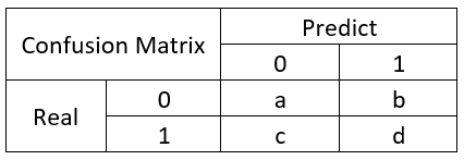
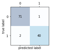
6.1 混淆矩陣及其實現(xiàn)
混淆矩陣,大家應(yīng)該都有聽說過,大致就是長下面這樣子的:
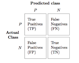
所以,有幾個概念需要先說明:
TP(True Positive): 真實為0,預(yù)測也為0
FN(False Negative): 真實為0,預(yù)測為1
FP(False Positive): 真實為1,預(yù)測為0
TN(True Negative): 真實為1,預(yù)測也為1
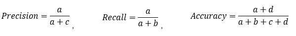
所以,衍生了幾個常用的指標(biāo):
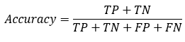 : 分類模型總體判斷的準(zhǔn)確率(包括了所有class的總體準(zhǔn)確率)
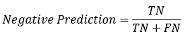
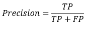 : 預(yù)測為0的準(zhǔn)確率
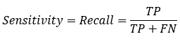 : 真實為0的準(zhǔn)確率
 : 真實為1的準(zhǔn)確率
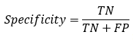
 : 預(yù)測為1的準(zhǔn)確率
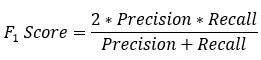 :?對于某個分類,綜合了Precision和Recall的一個判斷指標(biāo),F(xiàn)1-Score的值是從0到1的,1是最好,0是最差
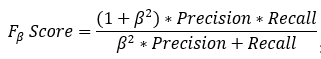 : 另外一個綜合Precision和Recall的標(biāo)準(zhǔn),F(xiàn)1-Score的變形
再舉個例子:
混淆矩陣網(wǎng)絡(luò)上有很多文章,也不用說刻意地去背去記,需要的時候百度一下你就知道,混淆矩陣實現(xiàn)代碼:
1from?sklearn.metrics?import?confusion_matrix
2
3pipe_svc.fit(X_train,?y_train)
4y_pred?=?pipe_svc.predict(X_test)
5confmat?=?confusion_matrix(y_true=y_test,?y_pred=y_pred)
6print(confmat)
output:
[[71  1]
 [ 2 40]]
 1fig,?ax?=?plt.subplots(figsize=(2.5,?2.5))
 2ax.matshow(confmat,?cmap=plt.cm.Blues,?alpha=0.3)
 3for?i?in?range(confmat.shape[0]):
 4????for?j?in?range(confmat.shape[1]):
 5????????ax.text(x=j,?y=i,?s=confmat[i,?j],?va='center',?ha='center')
 6
 7plt.xlabel('predicted?label')
 8plt.ylabel('true?label')
 9
10plt.tight_layout()
11plt.show()
6.2 相關(guān)評價指標(biāo)實現(xiàn)
分別是準(zhǔn)確度、recall以及F1指標(biāo)的實現(xiàn)。
1from?sklearn.metrics?import?precision_score,?recall_score,?f1_score
2
3print('Precision:?%.3f'?%?precision_score(y_true=y_test,?y_pred=y_pred))
4print('Recall:?%.3f'?%?recall_score(y_true=y_test,?y_pred=y_pred))
5print('F1:?%.3f'?%?f1_score(y_true=y_test,?y_pred=y_pred))
Precision: 0.976
Recall: 0.952
F1: 0.964
指定評價指標(biāo)自動選出最優(yōu)模型:
可以通過在make_scorer中設(shè)定參數(shù),確定需要用來評價的指標(biāo)(這里用了fl_score),這個函數(shù)可以直接輸出結(jié)果。
 1from?sklearn.metrics?import?make_scorer
 2
 3scorer?=?make_scorer(f1_score,?pos_label=0)
 4
 5c_gamma_range?=?[0.01,?0.1,?1.0,?10.0]
 6
 7param_grid?=?[{'clf__C':?c_gamma_range,
 8???????????????'clf__kernel':?['linear']},
 9??????????????{'clf__C':?c_gamma_range,
10???????????????'clf__gamma':?c_gamma_range,
11???????????????'clf__kernel':?['rbf']}]
12
13gs?=?GridSearchCV(estimator=pipe_svc,
14??????????????????param_grid=param_grid,
15??????????????????scoring=scorer,
16??????????????????cv=10,
17??????????????????n_jobs=-1)
18gs?=?gs.fit(X_train,?y_train)
19print(gs.best_score_)
20print(gs.best_params_)
0.982798668208
{'clf__C': 0.1, 'clf__kernel': 'linear'}
6.3 ROC曲線及其實現(xiàn)
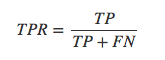
如果需要理解ROC曲線,那你就需要先了解一下混淆矩陣了,具體的內(nèi)容可以查看一下之前的文章,這里重點引入2個概念:
真正率(true positive rate,TPR),指的是被模型正確預(yù)測的正樣本的比例:
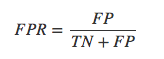
假正率(false positive rate,FPR) ,指的是被模型錯誤預(yù)測的正樣本的比例:
ROC曲線概念:
ROC(receiver operating characteristic)接受者操作特征,其顯示的是分類器的真正率和假正率之間的關(guān)系,如下圖所示:

ROC曲線有助于比較不同分類器的相對性能,其曲線下方的面積為AUC(area under curve),其面積越大則分類的性能越好,理想的分類器auc=1。
ROC曲線繪制:
對于一個特定的分類器和測試數(shù)據(jù)集,顯然只能得到一個分類結(jié)果,即一組FPR和TPR結(jié)果,而要得到一個曲線,我們實際上需要一系列FPR和TPR的值。
那么如何處理?很簡單,我們可以根據(jù)模型預(yù)測的概率值,并且設(shè)置不同的閾值來獲得不同的預(yù)測結(jié)果。什么意思?
比如說:
5個樣本,真實的target(目標(biāo)標(biāo)簽)是y=c(1,1,0,0,1)
模型分類器將預(yù)測樣本為1的概率p=c(0.5,0.6,0.55,0.4,0.7)
我們需要選定閾值才能把概率轉(zhuǎn)化為類別,
如果我們選定閾值為0.1,那么5個樣本被分進1的類別
如果選定0.3,結(jié)果仍然一樣
如果選了0.45作為閾值,那么只有樣本4被分進0
之后把所有得到的所有分類結(jié)果計算FTR,PTR,并繪制成線,就可以得到ROC曲線了,當(dāng)threshold(閾值)取值越多,ROC曲線越平滑。
ROC曲線代碼實現(xiàn):
 1from?sklearn.metrics?import?roc_curve,?auc
 2from?scipy?import?interp
 3
 4pipe_lr?=?Pipeline([('scl',?StandardScaler()),
 5????????????????????('pca',?PCA(n_components=2)),
 6????????????????????('clf',?LogisticRegression(penalty='l2',?
 7???????????????????????????????????????????????random_state=0,?
 8???????????????????????????????????????????????C=100.0))])
 9 ?
10X_train2?=?X_train[:,?[4,?14]]
11 ? # 因為全部特征丟進去的話,預(yù)測效果太好,畫ROC曲線不好看哈哈哈,所以只是取了2個特征
12
13
14cv?=?list(StratifiedKFold(n_splits=3,?
15??????????????????????????????random_state=1).split(X_train,?y_train))
16
17fig?=?plt.figure(figsize=(7,?5))
18
19mean_tpr?=?0.0
20mean_fpr?=?np.linspace(0,?1,?100)
21all_tpr?=?[]
22
23for?i,?(train,?test)?in?enumerate(cv):
24????probas?=?pipe_lr.fit(X_train2[train],
25?????????????????????????y_train[train]).predict_proba(X_train2[test])
26
27????fpr,?tpr,?thresholds?=?roc_curve(y_train[test],
28?????????????????????????????????????probas[:,?1],
29?????????????????????????????????????pos_label=1)
30????mean_tpr?+=?interp(mean_fpr,?fpr,?tpr)
31????mean_tpr[0]?=?0.0
32????roc_auc?=?auc(fpr,?tpr)
33????plt.plot(fpr,
34?????????????tpr,
35?????????????lw=1,
36?????????????label='ROC?fold?%d?(area?=?%0.2f)'
37???????????????????%?(i+1,?roc_auc))
38
39plt.plot([0,?1],
40?????????[0,?1],
41?????????linestyle='--',
42?????????color=(0.6,?0.6,?0.6),
43?????????label='random?guessing')
44
45mean_tpr?/=?len(cv)
46mean_tpr[-1]?=?1.0
47mean_auc?=?auc(mean_fpr,?mean_tpr)
48plt.plot(mean_fpr,?mean_tpr,?'k--',
49?????????label='mean?ROC?(area?=?%0.2f)'?%?mean_auc,?lw=2)
50plt.plot([0,?0,?1],
51?????????[0,?1,?1],
52?????????lw=2,
53?????????linestyle=':',
54?????????color='black',
55?????????label='perfect?performance')
56
57plt.xlim([-0.05,?1.05])
58plt.ylim([-0.05,?1.05])
59plt.xlabel('false?positive?rate')
60plt.ylabel('true?positive?rate')
61plt.title('Receiver?Operator?Characteristic')
62plt.legend(loc="lower?right")
63
64plt.tight_layout()
65plt.show()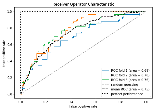
查看下AUC和準(zhǔn)確率的結(jié)果:
1pipe_lr?=?pipe_lr.fit(X_train2,?y_train)
2y_labels?=?pipe_lr.predict(X_test[:,?[4,?14]])
3y_probas?=?pipe_lr.predict_proba(X_test[:,?[4,?14]])[:,?1]
4#?note?that?we?use?probabilities?for?roc_auc
5#?the?`[:,?1]`?selects?the?positive?class?label?only
1from?sklearn.metrics?import?roc_auc_score,?accuracy_score
2print('ROC?AUC:?%.3f'?%?roc_auc_score(y_true=y_test,?y_score=y_probas))
3print('Accuracy:?%.3f'?%?accuracy_score(y_true=y_test,?y_pred=y_labels))
ROC AUC: 0.752
Accuracy: 0.711
往期精彩:
【原創(chuàng)首發(fā)】機器學(xué)習(xí)公式推導(dǎo)與代碼實現(xiàn)30講.pdf
【原創(chuàng)首發(fā)】深度學(xué)習(xí)語義分割理論與實戰(zhàn)指南.pdf

喜歡您就點個在看!