
溫州大學(xué)《機(jī)器學(xué)習(xí)》課程代碼(二)(回歸)
溫州大學(xué)《機(jī)器學(xué)習(xí)》課程代碼(二)(回歸)
代碼修改并注釋:黃海廣,[email protected]
下載地址:https://github.com/fengdu78/WZU-machine-learning-course
單變量線性回歸
import numpy as np
import pandas as pd
import matplotlib.pyplot as plt
import matplotlib.pyplot as plt
plt.rcParams['font.sans-serif']=['SimHei'] #用來(lái)正常顯示中文標(biāo)簽
plt.rcParams['axes.unicode_minus']=False #用來(lái)正常顯示負(fù)號(hào)
path = 'data/regress_data1.csv'
data = pd.read_csv(path)
data.head()
| 人口 | 收益 | |
|---|---|---|
| 0 | 6.1101 | 17.5920 |
| 1 | 5.5277 | 9.1302 |
| 2 | 8.5186 | 13.6620 |
| 3 | 7.0032 | 11.8540 |
| 4 | 5.8598 | 6.8233 |
data.describe()
| 人口 | 收益 | |
|---|---|---|
| count | 97.000000 | 97.000000 |
| mean | 8.159800 | 5.839135 |
| std | 3.869884 | 5.510262 |
| min | 5.026900 | -2.680700 |
| 25% | 5.707700 | 1.986900 |
| 50% | 6.589400 | 4.562300 |
| 75% | 8.578100 | 7.046700 |
| max | 22.203000 | 24.147000 |
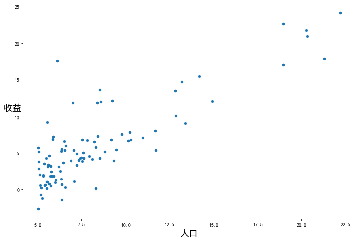
看下數(shù)據(jù)長(zhǎng)什么樣子
data.plot(kind='scatter', x='人口', y='收益', figsize=(12,8))
plt.xlabel('人口', fontsize=18)
plt.ylabel('收益', rotation=0, fontsize=18)
plt.show()
現(xiàn)在讓我們使用梯度下降來(lái)實(shí)現(xiàn)線性回歸,以最小化代價(jià)函數(shù)。
首先,我們將創(chuàng)建一個(gè)以參數(shù)為特征函數(shù)的代價(jià)函數(shù)
其中:
def computeCost(X, y, w):
    inner = np.power(((X * w.T) - y), 2)# (m,n) @ (n, 1) -> (n, 1)
#     return np.sum(inner) / (2 * len(X))
    return np.sum(inner) / (2 * X.shape[0])
讓我們?cè)谟?xùn)練集中添加一列,以便我們可以使用向量化的解決方案來(lái)計(jì)算代價(jià)和梯度。
data.insert(0, 'Ones', 1)
data
| Ones | 人口 | 收益 | |
|---|---|---|---|
| 0 | 1 | 6.1101 | 17.59200 |
| 1 | 1 | 5.5277 | 9.13020 |
| 2 | 1 | 8.5186 | 13.66200 |
| 3 | 1 | 7.0032 | 11.85400 |
| 4 | 1 | 5.8598 | 6.82330 |
| ... | ... | ... | ... |
| 92 | 1 | 5.8707 | 7.20290 |
| 93 | 1 | 5.3054 | 1.98690 |
| 94 | 1 | 8.2934 | 0.14454 |
| 95 | 1 | 13.3940 | 9.05510 |
| 96 | 1 | 5.4369 | 0.61705 |
97 rows × 3 columns
現(xiàn)在我們來(lái)做一些變量初始化。
# set X (training data) and y (target variable)
cols = data.shape[1]
X = data.iloc[:,:cols-1]#X是所有行,去掉最后一列
y = data.iloc[:,cols-1:]#X是所有行,最后一列
觀察下 X (訓(xùn)練集) and y (目標(biāo)變量)是否正確.
X.head()#head()是觀察前5行
| Ones | 人口 | |
|---|---|---|
| 0 | 1 | 6.1101 |
| 1 | 1 | 5.5277 |
| 2 | 1 | 8.5186 |
| 3 | 1 | 7.0032 |
| 4 | 1 | 5.8598 |
y.head()
| 收益 | |
|---|---|
| 0 | 17.5920 |
| 1 | 9.1302 |
| 2 | 13.6620 |
| 3 | 11.8540 |
| 4 | 6.8233 |
代價(jià)函數(shù)是應(yīng)該是numpy矩陣,所以我們需要轉(zhuǎn)換X和Y,然后才能使用它們。我們還需要初始化w。
X = np.matrix(X.values)
y = np.matrix(y.values)
w = np.matrix(np.array([0,0]))
w 是一個(gè)(1,2)矩陣
w
matrix([[0, 0]])
看下維度
X.shape, w.shape, y.shape
((97, 2), (1, 2), (97, 1))
計(jì)算代價(jià)函數(shù) (theta初始值為0).
computeCost(X, y, w)
32.072733877455676
Batch Gradient Decent(批量梯度下降)
def batch_gradientDescent(X, y, w, alpha, iters):
    temp = np.matrix(np.zeros(w.shape))
    parameters = int(w.ravel().shape[1])
    cost = np.zeros(iters)

    for i in range(iters):
        error = (X * w.T) - y

        for j in range(parameters):
            term = np.multiply(error, X[:, j])
            temp[0, j] = w[0, j] - ((alpha / len(X)) * np.sum(term))

        w = temp
        cost[i] = computeCost(X, y, w)

    return w, cost
初始化一些附加變量 - 學(xué)習(xí)速率α和要執(zhí)行的迭代次數(shù)。
alpha = 0.01
iters = 1000
現(xiàn)在讓我們運(yùn)行梯度下降算法來(lái)將我們的參數(shù)θ適合于訓(xùn)練集。
g, cost = batch_gradientDescent(X, y, w, alpha, iters)
g
matrix([[-3.24140214, 1.1272942 ]])
最后,我們可以使用我們擬合的參數(shù)計(jì)算訓(xùn)練模型的代價(jià)函數(shù)(誤差)。
computeCost(X, y, g)
4.515955503078912
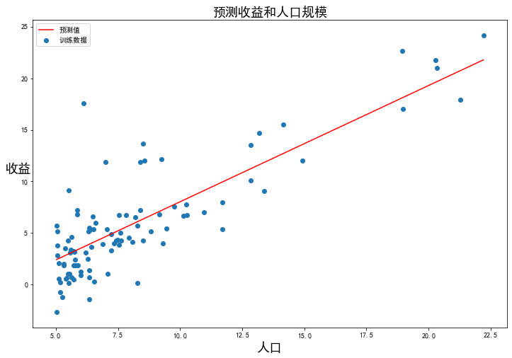
現(xiàn)在我們來(lái)繪制線性模型以及數(shù)據(jù),直觀地看出它的擬合。
x = np.linspace(data['人口'].min(), data['人口'].max(), 100)
f = g[0, 0] + (g[0, 1] * x)

fig, ax = plt.subplots(figsize=(12, 8))
ax.plot(x, f, 'r', label='預(yù)測(cè)值')
ax.scatter(data['人口'], data['收益'], label='訓(xùn)練數(shù)據(jù)')
ax.legend(loc=2)
ax.set_xlabel('人口', fontsize=18)
ax.set_ylabel('收益', rotation=0, fontsize=18)
ax.set_title('預(yù)測(cè)收益和人口規(guī)模', fontsize=18)
plt.show()
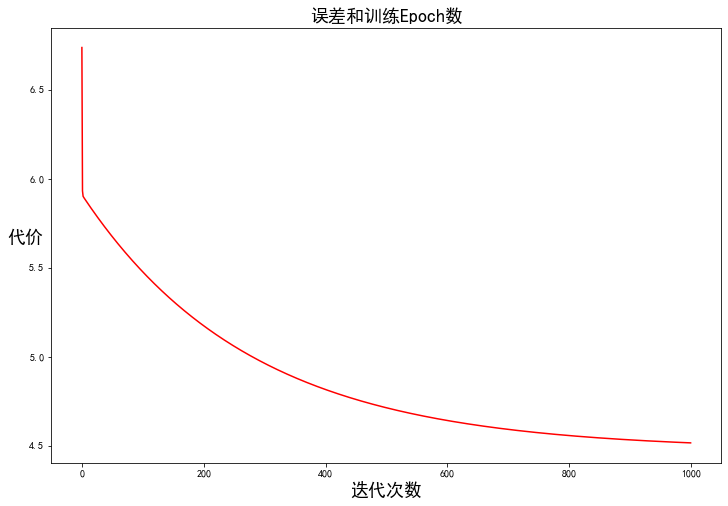
由于梯度方程式函數(shù)也在每個(gè)訓(xùn)練迭代中輸出一個(gè)代價(jià)的向量,所以我們也可以繪制。請(qǐng)注意,代價(jià)總是降低 - 這是凸優(yōu)化問題的一個(gè)例子。
fig, ax = plt.subplots(figsize=(12, 8))
ax.plot(np.arange(iters), cost, 'r')
ax.set_xlabel('迭代次數(shù)', fontsize=18)
ax.set_ylabel('代價(jià)', rotation=0, fontsize=18)
ax.set_title('誤差和訓(xùn)練Epoch數(shù)', fontsize=18)
plt.show()
多變量線性回歸
練習(xí)還包括一個(gè)房屋價(jià)格數(shù)據(jù)集,其中有2個(gè)變量(房子的大小,臥室的數(shù)量)和目標(biāo)(房子的價(jià)格)。我們使用我們已經(jīng)應(yīng)用的技術(shù)來(lái)分析數(shù)據(jù)集。
path = 'data/regress_data2.csv'
data2 = pd.read_csv(path)
data2.head()
| 面積 | 房間數(shù) | 價(jià)格 | |
|---|---|---|---|
| 0 | 2104 | 3 | 399900 |
| 1 | 1600 | 3 | 329900 |
| 2 | 2400 | 3 | 369000 |
| 3 | 1416 | 2 | 232000 |
| 4 | 3000 | 4 | 539900 |
對(duì)于此任務(wù),我們添加了另一個(gè)預(yù)處理步驟 - 特征歸一化。這個(gè)對(duì)于pandas來(lái)說(shuō)很簡(jiǎn)單
data2 = (data2 - data2.mean()) / data2.std()
data2.head()
| 面積 | 房間數(shù) | 價(jià)格 | |
|---|---|---|---|
| 0 | 0.130010 | -0.223675 | 0.475747 |
| 1 | -0.504190 | -0.223675 | -0.084074 |
| 2 | 0.502476 | -0.223675 | 0.228626 |
| 3 | -0.735723 | -1.537767 | -0.867025 |
| 4 | 1.257476 | 1.090417 | 1.595389 |
現(xiàn)在我們重復(fù)第1部分的預(yù)處理步驟,并對(duì)新數(shù)據(jù)集運(yùn)行線性回歸程序。
# add ones column
data2.insert(0, 'Ones', 1)

# set X (training data) and y (target variable)
cols = data2.shape[1]
X2 = data2.iloc[:,0:cols-1]
y2 = data2.iloc[:,cols-1:cols]

# convert to matrices and initialize theta
X2 = np.matrix(X2.values)
y2 = np.matrix(y2.values)
w2 = np.matrix(np.array([0,0,0]))

# perform linear regression on the data set
g2, cost2 = batch_gradientDescent(X2, y2, w2, alpha, iters)

# get the cost (error) of the model
computeCost(X2, y2, g2)
0.13070336960771892
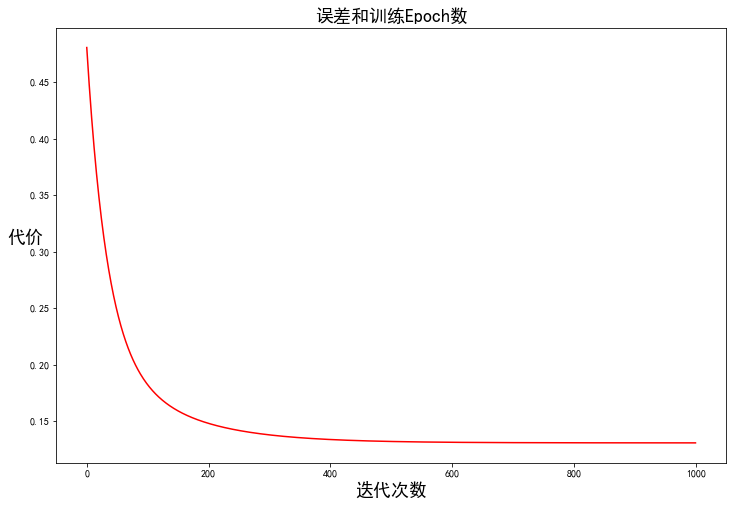
我們也可以快速查看這一個(gè)的訓(xùn)練進(jìn)程。
fig, ax = plt.subplots(figsize=(12,8))
ax.plot(np.arange(iters), cost2, 'r')
ax.set_xlabel('迭代次數(shù)', fontsize=18)
ax.set_ylabel('代價(jià)', rotation=0, fontsize=18)
ax.set_title('誤差和訓(xùn)練Epoch數(shù)', fontsize=18)
plt.show()
我們也可以使用scikit-learn的線性回歸函數(shù),而不是從頭開始實(shí)現(xiàn)這些算法。我們將scikit-learn的線性回歸算法應(yīng)用于第1部分的數(shù)據(jù),并看看它的表現(xiàn)。
from sklearn.linear_model import LinearRegression
model = LinearRegression()
model.fit(X, y)
LinearRegression()
scikit-learn model的預(yù)測(cè)表現(xiàn)
x = np.array(X[:, 1].A1)
f = model.predict(X).flatten()

fig, ax = plt.subplots(figsize=(12, 8))
ax.plot(x, f, 'r', label='預(yù)測(cè)值')
ax.scatter(data['人口'], data['收益'], label='訓(xùn)練數(shù)據(jù)')
ax.legend(loc=2, fontsize=18)
ax.set_xlabel('人口', fontsize=18)
ax.set_ylabel('收益', rotation=0, fontsize=18)
ax.set_title('預(yù)測(cè)收益和人口規(guī)模', fontsize=18)
plt.show()

正則化
,此時(shí)稱作Ridge Regression:
from sklearn.linear_model import Ridge
model = Ridge()
model.fit(X, y)
Ridge()
x2 = np.array(X[:, 1].A1)
f2 = model.predict(X).flatten()

fig, ax = plt.subplots(figsize=(12, 8))
ax.plot(x2, f2, 'r', label='預(yù)測(cè)值Ridge')
ax.scatter(data['人口'], data['收益'], label='訓(xùn)練數(shù)據(jù)')
ax.legend(loc=2, fontsize=18)
ax.set_xlabel('人口', fontsize=18)
ax.set_ylabel('收益', rotation=0, fontsize=18)
ax.set_title('預(yù)測(cè)收益和人口規(guī)模', fontsize=18)
plt.show()

正則化:
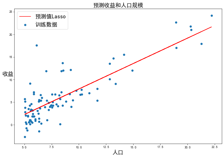
,此時(shí)稱作Lasso Regression
from sklearn.linear_model import Lasso
model = Lasso()
model.fit(X, y)
Lasso()
x3= np.array(X[:, 1].A1)
f3 = model.predict(X).flatten()

fig, ax = plt.subplots(figsize=(12, 8))
ax.plot(x3, f3, 'r', label='預(yù)測(cè)值Lasso')
ax.scatter(data['人口'], data['收益'], label='訓(xùn)練數(shù)據(jù)')
ax.legend(loc=2, fontsize=18)
ax.set_xlabel('人口', fontsize=18)
ax.set_ylabel('收益', rotation=0, fontsize=18)
ax.set_title('預(yù)測(cè)收益和人口規(guī)模', fontsize=18)
plt.show()
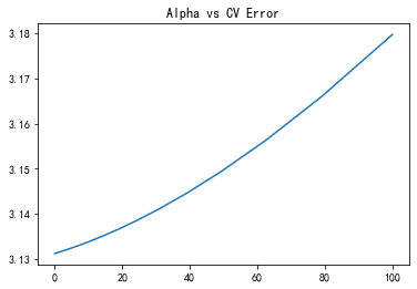
調(diào)參
from sklearn.model_selection import cross_val_score
alphas = np.logspace(-3, 2, 50)
test_scores = []
for alpha in alphas:
    clf = Ridge(alpha)
    test_score = np.sqrt(-cross_val_score(clf, X, y, cv=5, scoring='neg_mean_squared_error'))
    test_scores.append(np.mean(test_score))
import matplotlib.pyplot as plt
plt.plot(alphas, test_scores)
plt.title("Alpha vs CV Error");
plt.show()
最小二乘法(LSM)
最小二乘法的需要求解最優(yōu)參數(shù):
已知:目標(biāo)函數(shù)
其中:
將向量表達(dá)形式轉(zhuǎn)為矩陣表達(dá)形式,則有 ,其中為行列的矩陣(為樣本個(gè)數(shù),為特征個(gè)數(shù)),為行1列的矩陣(包含了),為行1列的矩陣,則可以求得最優(yōu)參數(shù)
梯度下降與最小二乘法的比較:
梯度下降: 需要選擇學(xué)習(xí)率,需要多次迭代,當(dāng)特征數(shù)量大時(shí)也能較好適用,適用于各種類型的模型
最小二乘法: 不需要選擇學(xué)習(xí)率,一次計(jì)算得出,需要計(jì)算,如果特征數(shù)量較大則運(yùn)算代價(jià)大,因?yàn)榫仃嚹娴挠?jì)算時(shí)間復(fù)雜度為,通常來(lái)說(shuō)當(dāng)小于10000 時(shí)還是可以接受的,只適用于線性模型,不適合邏輯回歸模型等其他模型
# 正規(guī)方程
def LSM(X, y):
    w = np.linalg.inv(X.T@X)@X.T@y#X.T@X等價(jià)于X.T.dot(X)
    return w
final_w2=LSM(X, y)#感覺和批量梯度下降的theta的值有點(diǎn)差距
final_w2
matrix([[-3.89578088],
        [ 1.19303364]])
#梯度下降得到的結(jié)果是matrix([[-3.24140214, 1.1272942 ]])
參考
機(jī)器學(xué)習(xí),吳恩達(dá) 《統(tǒng)計(jì)學(xué)習(xí)方法》,李航 機(jī)器學(xué)習(xí)課程,鄒博
往期精彩回顧
本站qq群851320808,加入微信群請(qǐng)掃碼: