
【深度學(xué)習(xí)】使用transformer進(jìn)行圖像分類
文章目錄
1、導(dǎo)入模型
2、定義加載函數(shù)
3、定義批量加載函數(shù)
4、加載數(shù)據(jù)
5、定義數(shù)據(jù)預(yù)處理及訓(xùn)練模型的一些超參數(shù)
6、定義數(shù)據(jù)增強(qiáng)模型
7、構(gòu)建模型
7.1 構(gòu)建多層感知器(MLP)
7.2 創(chuàng)建一個(gè)類似卷積層的patch層
7.3 查看由patch層隨機(jī)生成的圖像塊
7.4構(gòu)建patch 編碼層( encoding layer)
7.5構(gòu)建ViT模型
8、編譯、訓(xùn)練模型
9、查看運(yùn)行結(jié)果
使用Transformer來(lái)提升模型的性能
最近幾年,Transformer體系結(jié)構(gòu)已成為自然語(yǔ)言處理任務(wù)的實(shí)際標(biāo)準(zhǔn),
但其在計(jì)算機(jī)視覺(jué)中的應(yīng)用還受到限制。在視覺(jué)上,注意力要么與卷積網(wǎng)絡(luò)結(jié)合使用,
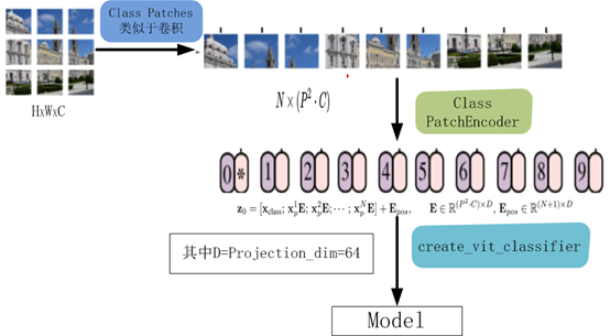
要么用于替換卷積網(wǎng)絡(luò)的某些組件,同時(shí)將其整體結(jié)構(gòu)保持在適當(dāng)?shù)奈恢谩?020年10月22日,谷歌人工智能研究院發(fā)表一篇題為“An Image is Worth 16x16 Words: Transformers for Image Recognition at Scale”的文章。文章將圖像切割成一個(gè)個(gè)圖像塊,組成序列化的數(shù)據(jù)輸入Transformer執(zhí)行圖像分類任務(wù)。當(dāng)對(duì)大量數(shù)據(jù)進(jìn)行預(yù)訓(xùn)練并將其傳輸?shù)蕉鄠€(gè)中型或小型圖像識(shí)別數(shù)據(jù)集(如ImageNet、CIFAR-100、VTAB等)時(shí),與目前的卷積網(wǎng)絡(luò)相比,Vision Transformer(ViT)獲得了出色的結(jié)果,同時(shí)所需的計(jì)算資源也大大減少。
這里我們以ViT我模型,實(shí)現(xiàn)對(duì)數(shù)據(jù)CiFar10的分類工作,模型性能得到進(jìn)一步的提升。
1、導(dǎo)入模型
import osimport mathimport numpy as npimport pickle as pimport tensorflow as tffrom tensorflow import kerasimport matplotlib.pyplot as pltfrom tensorflow.keras import layersimport tensorflow_addons as tfa%matplotlib inline
這里使用了TensorFlow_addons模塊,它實(shí)現(xiàn)了核心 TensorFlow 中未提供的新功能。
tensorflow_addons的安裝要注意與tf的版本對(duì)應(yīng)關(guān)系,請(qǐng)參考:
https://github.com/tensorflow/addons。
安裝addons時(shí)要注意其版本與tensorflow版本的對(duì)應(yīng),具體關(guān)系以上這個(gè)鏈接有。
2、定義加載函數(shù)
def load_CIFAR_data(data_dir):"""load CIFAR data"""images_train=[]labels_train=[]for i in range(5):f=os.path.join(data_dir,'data_batch_%d' % (i+1))print('loading ',f)# 調(diào)用 load_CIFAR_batch( )獲得批量的圖像及其對(duì)應(yīng)的標(biāo)簽image_batch,label_batch=load_CIFAR_batch(f)images_train.append(image_batch)labels_train.append(label_batch)Xtrain=np.concatenate(images_train)Ytrain=np.concatenate(labels_train)del image_batch ,label_batchXtest,Ytest=load_CIFAR_batch(os.path.join(data_dir,'test_batch'))print('finished loadding CIFAR-10 data')# 返回訓(xùn)練集的圖像和標(biāo)簽,測(cè)試集的圖像和標(biāo)簽return (Xtrain,Ytrain),(Xtest,Ytest)
3、定義批量加載函數(shù)
def load_CIFAR_batch(filename):""" load single batch of cifar """with open(filename, 'rb')as f:# 一個(gè)樣本由標(biāo)簽和圖像數(shù)據(jù)組成# (3072=32x32x3)# ...#data_dict = p.load(f, encoding='bytes')images= data_dict[b'data']labels = data_dict[b'labels']# 把原始數(shù)據(jù)結(jié)構(gòu)調(diào)整為: BCWHimages = images.reshape(10000, 3, 32, 32)# tensorflow處理圖像數(shù)據(jù)的結(jié)構(gòu):BWHC# 把通道數(shù)據(jù)C移動(dòng)到最后一個(gè)維度images = images.transpose (0,2,3,1)labels = np.array(labels)return images, labels
4、加載數(shù)據(jù)
data_dir = r'C:\Users\wumg\jupyter-ipynb\data\cifar-10-batches-py'(x_train,y_train),(x_test,y_test) = load_CIFAR_data(data_dir)
把數(shù)據(jù)轉(zhuǎn)換為dataset格式
train_dataset = tf.data.Dataset.from_tensor_slices((x_train, y_train))test_dataset = tf.data.Dataset.from_tensor_slices((x_test, y_test))
5、定義數(shù)據(jù)預(yù)處理及訓(xùn)練模型的一些超參數(shù)
num_classes = 10input_shape = (32, 32, 3)learning_rate = 0.001weight_decay = 0.0001batch_size = 256num_epochs = 10image_size = 72 # We'll resize input images to this sizepatch_size = 6 # Size of the patches to be extract from the input imagesnum_patches = (image_size // patch_size) ** 2projection_dim = 64num_heads = 4transformer_units = [projection_dim * 2,projection_dim,] # Size of the transformer layerstransformer_layers = 8mlp_head_units = [2048, 1024] # Size of the dense layers of the final classifier
6、定義數(shù)據(jù)增強(qiáng)模型
data_augmentation = keras.Sequential([layers.experimental.preprocessing.Normalization(),layers.experimental.preprocessing.Resizing(image_size, image_size),layers.experimental.preprocessing.RandomFlip("horizontal"),layers.experimental.preprocessing.RandomRotation(factor=0.02),layers.experimental.preprocessing.RandomZoom(height_factor=0.2, width_factor=0.2),],name="data_augmentation",)# 使預(yù)處理層的狀態(tài)與正在傳遞的數(shù)據(jù)相匹配#Compute the mean and the variance of the training data for normalization.data_augmentation.layers[0].adapt(x_train)
預(yù)處理層是在模型訓(xùn)練開(kāi)始之前計(jì)算其狀態(tài)的層。他們?cè)谟?xùn)練期間不會(huì)得到更新。大多數(shù)預(yù)處理層為狀態(tài)計(jì)算實(shí)現(xiàn)了adapt()方法。
adapt(data, batch_size=None, steps=None, reset_state=True)該函數(shù)參數(shù)說(shuō)明如下:

7、構(gòu)建模型
7.1 構(gòu)建多層感知器(MLP)
def mlp(x, hidden_units, dropout_rate):for units in hidden_units:x = layers.Dense(units, activation=tf.nn.gelu)(x)x = layers.Dropout(dropout_rate)(x)return x
7.2 創(chuàng)建一個(gè)類似卷積層的patch層
class Patches(layers.Layer):def __init__(self, patch_size):super(Patches, self).__init__()self.patch_size = patch_sizedef call(self, images):batch_size = tf.shape(images)[0]patches = tf.image.extract_patches(images=images,sizes=[1, self.patch_size, self.patch_size, 1],strides=[1, self.patch_size, self.patch_size, 1],rates=[1, 1, 1, 1],padding="VALID",)patch_dims = patches.shape[-1]patches = tf.reshape(patches, [batch_size, -1, patch_dims])return patches
7.3 查看由patch層隨機(jī)生成的圖像塊
import matplotlib.pyplot as pltplt.figure(figsize=(4, 4))image = x_train[np.random.choice(range(x_train.shape[0]))]plt.imshow(image.astype("uint8"))plt.axis("off")resized_image = tf.image.resize(tf.convert_to_tensor([image]), size=(image_size, image_size))patches = Patches(patch_size)(resized_image)print(f"Image size: {image_size} X {image_size}")print(f"Patch size: {patch_size} X {patch_size}")print(f"Patches per image: {patches.shape[1]}")print(f"Elements per patch: {patches.shape[-1]}")n = int(np.sqrt(patches.shape[1]))plt.figure(figsize=(4, 4))for i, patch in enumerate(patches[0]):ax = plt.subplot(n, n, i + 1)patch_img = tf.reshape(patch, (patch_size, patch_size, 3))plt.imshow(patch_img.numpy().astype("uint8"))plt.axis("off")
運(yùn)行結(jié)果
Image size: 72 X 72
Patch size: 6 X 6
Patches per image: 144
Elements per patch: 108


7.4構(gòu)建patch 編碼層( encoding layer)
class PatchEncoder(layers.Layer):def __init__(self, num_patches, projection_dim):super(PatchEncoder, self).__init__()self.num_patches = num_patches#一個(gè)全連接層,其輸出維度為projection_dim,沒(méi)有指明激活函數(shù)self.projection = layers.Dense(units=projection_dim)#定義一個(gè)嵌入層,這是一個(gè)可學(xué)習(xí)的層#輸入維度為num_patches,輸出維度為projection_dimself.position_embedding = layers.Embedding(input_dim=num_patches, output_dim=projection_dim)def call(self, patch):positions = tf.range(start=0, limit=self.num_patches, delta=1)encoded = self.projection(patch) + self.position_embedding(positions)return encoded
7.5構(gòu)建ViT模型
def create_vit_classifier():inputs = layers.Input(shape=input_shape)# Augment data.augmented = data_augmentation(inputs)#augmented = augmented_train_batches(inputs)# Create patches.patches = Patches(patch_size)(augmented)# Encode patches.encoded_patches = PatchEncoder(num_patches, projection_dim)(patches)# Create multiple layers of the Transformer block.for _ in range(transformer_layers):# Layer normalization 1.x1 = layers.LayerNormalization(epsilon=1e-6)(encoded_patches)# Create a multi-head attention layer.attention_output = layers.MultiHeadAttention(num_heads=num_heads, key_dim=projection_dim, dropout=0.1x1)# Skip connection 1.x2 = layers.Add()([attention_output, encoded_patches])# Layer normalization 2.x3 = layers.LayerNormalization(epsilon=1e-6)(x2)# MLP.x3 = mlp(x3, hidden_units=transformer_units, dropout_rate=0.1)# Skip connection 2.encoded_patches = layers.Add()([x3, x2])# Create a [batch_size, projection_dim] tensor.representation = layers.LayerNormalization(epsilon=1e-6)(encoded_patches)representation = layers.Flatten()(representation)representation = layers.Dropout(0.5)(representation)# Add MLP.features = mlp(representation, hidden_units=mlp_head_units, dropout_rate=0.5)# Classify outputs.logits = layers.Dense(num_classes)(features)# Create the Keras model.model = keras.Model(inputs=inputs, outputs=logits)return model
該模型的處理流程如下圖所示
8、編譯、訓(xùn)練模型
def run_experiment(model):optimizer = tfa.optimizers.AdamW(learning_rate=learning_rate, weight_decay=weight_decay)model.compile(optimizer=optimizer,loss=keras.losses.SparseCategoricalCrossentropy(from_logits=True),metrics=[="accuracy"),name="top-5-accuracy"),],)#checkpoint_filepath = r".\tmp\checkpoint"checkpoint_filepath ="model_bak.hdf5"checkpoint_callback = keras.callbacks.ModelCheckpoint(checkpoint_filepath,monitor="val_accuracy",save_best_only=True,save_weights_only=True,)history = model.fit(x=x_train,y=y_train,batch_size=batch_size,epochs=num_epochs,validation_split=0.1,callbacks=[checkpoint_callback],)model.load_weights(checkpoint_filepath)accuracy, top_5_accuracy = model.evaluate(x_test, y_test)accuracy: {round(accuracy * 100, 2)}%")top 5 accuracy: {round(top_5_accuracy * 100, 2)}%")return history
實(shí)例化類,運(yùn)行模型
vit_classifier = create_vit_classifier()history = run_experiment(vit_classifier)
運(yùn)行結(jié)果
Epoch 1/10
176/176 [==============================] - 68s 333ms/step - loss: 2.6394 - accuracy: 0.2501 - top-5-accuracy: 0.7377 - val_loss: 1.5331 - val_accuracy: 0.4580 - val_top-5-accuracy: 0.9092
Epoch 2/10
176/176 [==============================] - 58s 327ms/step - loss: 1.6359 - accuracy: 0.4150 - top-5-accuracy: 0.8821 - val_loss: 1.2714 - val_accuracy: 0.5348 - val_top-5-accuracy: 0.9464
Epoch 3/10
176/176 [==============================] - 58s 328ms/step - loss: 1.4332 - accuracy: 0.4839 - top-5-accuracy: 0.9210 - val_loss: 1.1633 - val_accuracy: 0.5806 - val_top-5-accuracy: 0.9616
Epoch 4/10
176/176 [==============================] - 58s 329ms/step - loss: 1.3253 - accuracy: 0.5280 - top-5-accuracy: 0.9349 - val_loss: 1.1010 - val_accuracy: 0.6112 - val_top-5-accuracy: 0.9572
Epoch 5/10
176/176 [==============================] - 58s 330ms/step - loss: 1.2380 - accuracy: 0.5626 - top-5-accuracy: 0.9411 - val_loss: 1.0212 - val_accuracy: 0.6400 - val_top-5-accuracy: 0.9690
Epoch 6/10
176/176 [==============================] - 58s 330ms/step - loss: 1.1486 - accuracy: 0.5945 - top-5-accuracy: 0.9520 - val_loss: 0.9698 - val_accuracy: 0.6602 - val_top-5-accuracy: 0.9718
Epoch 7/10
176/176 [==============================] - 58s 330ms/step - loss: 1.1208 - accuracy: 0.6060 - top-5-accuracy: 0.9558 - val_loss: 0.9215 - val_accuracy: 0.6724 - val_top-5-accuracy: 0.9790
Epoch 8/10
176/176 [==============================] - 58s 330ms/step - loss: 1.0643 - accuracy: 0.6248 - top-5-accuracy: 0.9621 - val_loss: 0.8709 - val_accuracy: 0.6944 - val_top-5-accuracy: 0.9768
Epoch 9/10
176/176 [==============================] - 58s 330ms/step - loss: 1.0119 - accuracy: 0.6446 - top-5-accuracy: 0.9640 - val_loss: 0.8290 - val_accuracy: 0.7142 - val_top-5-accuracy: 0.9784
Epoch 10/10
176/176 [==============================] - 58s 330ms/step - loss: 0.9740 - accuracy: 0.6615 - top-5-accuracy: 0.9666 - val_loss: 0.8175 - val_accuracy: 0.7096 - val_top-5-accuracy: 0.9806
313/313 [==============================] - 9s 27ms/step - loss: 0.8514 - accuracy: 0.7032 - top-5-accuracy: 0.9773
Test accuracy: 70.32%
Test top 5 accuracy: 97.73%
In [15]:
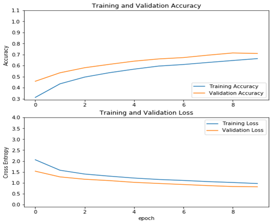
從結(jié)果看可以來(lái)看,測(cè)試精度已達(dá)70%,這是一個(gè)較大提升!
9、查看運(yùn)行結(jié)果
acc = history.history['accuracy']val_acc = history.history['val_accuracy']loss = history.history['loss']val_loss =history.history['val_loss']plt.figure(figsize=(8, 8))plt.subplot(2, 1, 1)plt.plot(acc, label='Training Accuracy')plt.plot(val_acc, label='Validation Accuracy')plt.legend(loc='lower right')plt.ylabel('Accuracy')plt.ylim([min(plt.ylim()),1.1])plt.title('Training and Validation Accuracy')plt.subplot(2, 1, 2)plt.plot(loss, label='Training Loss')plt.plot(val_loss, label='Validation Loss')plt.legend(loc='upper right')plt.ylabel('Cross Entropy')plt.ylim([-0.1,4.0])plt.title('Training and Validation Loss')plt.xlabel('epoch')plt.show()
運(yùn)行結(jié)果
作者 :吳茂貴,資深大數(shù)據(jù)和人工智能技術(shù)專家,在BI、數(shù)據(jù)挖掘與分析、數(shù)據(jù)倉(cāng)庫(kù)、機(jī)器學(xué)習(xí)等領(lǐng)域工作超過(guò)20年!在基于Spark、TensorFlow、Pytorch、Keras等機(jī)器學(xué)習(xí)和深度學(xué)習(xí)方面有大量的工程實(shí)踐經(jīng)驗(yàn)。代表作有《深入淺出Embedding:原理解析與應(yīng)用實(shí)踐》、《Python深度學(xué)習(xí)基于Pytorch》和《Python深度學(xué)習(xí)基于TensorFlow》。
——The End——
往期精彩回顧 本站qq群851320808,加入微信群請(qǐng)掃碼: