
使用transformer進行圖像分類
文章目錄
1、導入模型
2、定義加載函數
3、定義批量加載函數
4、加載數據
5、定義數據預處理及訓練模型的一些超參數
6、定義數據增強模型
7、構建模型
7.1 構建多層感知器(MLP)
7.2 創(chuàng)建一個類似卷積層的patch層
7.3 查看由patch層隨機生成的圖像塊
7.4構建patch 編碼層( encoding layer)
7.5構建ViT模型
8、編譯、訓練模型
9、查看運行結果
使用Transformer來提升模型的性能
最近幾年,Transformer體系結構已成為自然語言處理任務的實際標準,
但其在計算機視覺中的應用還受到限制。在視覺上,注意力要么與卷積網絡結合使用,
要么用于替換卷積網絡的某些組件,同時將其整體結構保持在適當的位置。2020年10月22日,谷歌人工智能研究院發(fā)表一篇題為“An Image is Worth 16x16 Words: Transformers for Image Recognition at Scale”的文章。文章將圖像切割成一個個圖像塊,組成序列化的數據輸入Transformer執(zhí)行圖像分類任務。當對大量數據進行預訓練并將其傳輸到多個中型或小型圖像識別數據集(如ImageNet、CIFAR-100、VTAB等)時,與目前的卷積網絡相比,Vision Transformer(ViT)獲得了出色的結果,同時所需的計算資源也大大減少。
這里我們以ViT我模型,實現(xiàn)對數據CiFar10的分類工作,模型性能得到進一步的提升。
1、導入模型
import osimport mathimport numpy as npimport pickle as pimport tensorflow as tffrom tensorflow import kerasimport matplotlib.pyplot as pltfrom tensorflow.keras import layersimport tensorflow_addons as tfa%matplotlib inline
這里使用了TensorFlow_addons模塊,它實現(xiàn)了核心 TensorFlow 中未提供的新功能。
tensorflow_addons的安裝要注意與tf的版本對應關系,請參考:
https://github.com/tensorflow/addons。
安裝addons時要注意其版本與tensorflow版本的對應,具體關系以上這個鏈接有。
2、定義加載函數
def load_CIFAR_data(data_dir):"""load CIFAR data"""images_train=[]labels_train=[]for i in range(5):f=os.path.join(data_dir,'data_batch_%d' % (i+1))print('loading ',f)# 調用 load_CIFAR_batch( )獲得批量的圖像及其對應的標簽image_batch,label_batch=load_CIFAR_batch(f)images_train.append(image_batch)labels_train.append(label_batch)Xtrain=np.concatenate(images_train)Ytrain=np.concatenate(labels_train)del image_batch ,label_batchXtest,Ytest=load_CIFAR_batch(os.path.join(data_dir,'test_batch'))print('finished loadding CIFAR-10 data')# 返回訓練集的圖像和標簽,測試集的圖像和標簽return (Xtrain,Ytrain),(Xtest,Ytest)
3、定義批量加載函數
def load_CIFAR_batch(filename):""" load single batch of cifar """with open(filename, 'rb')as f:# 一個樣本由標簽和圖像數據組成# (3072=32x32x3)# ...#data_dict = p.load(f, encoding='bytes')images= data_dict[b'data']labels = data_dict[b'labels']# 把原始數據結構調整為: BCWHimages = images.reshape(10000, 3, 32, 32)# tensorflow處理圖像數據的結構:BWHC# 把通道數據C移動到最后一個維度images = images.transpose (0,2,3,1)labels = np.array(labels)return images, labels
4、加載數據
data_dir = r'C:\Users\wumg\jupyter-ipynb\data\cifar-10-batches-py'(x_train,y_train),(x_test,y_test) = load_CIFAR_data(data_dir)
把數據轉換為dataset格式
train_dataset = tf.data.Dataset.from_tensor_slices((x_train, y_train))test_dataset = tf.data.Dataset.from_tensor_slices((x_test, y_test))
5、定義數據預處理及訓練模型的一些超參數
num_classes = 10input_shape = (32, 32, 3)learning_rate = 0.001weight_decay = 0.0001batch_size = 256num_epochs = 10image_size = 72 # We'll resize input images to this sizepatch_size = 6 # Size of the patches to be extract from the input imagesnum_patches = (image_size // patch_size) ** 2projection_dim = 64num_heads = 4transformer_units = [projection_dim * 2,projection_dim,] # Size of the transformer layerstransformer_layers = 8mlp_head_units = [2048, 1024] # Size of the dense layers of the final classifier
6、定義數據增強模型
data_augmentation = keras.Sequential([layers.experimental.preprocessing.Normalization(),layers.experimental.preprocessing.Resizing(image_size, image_size),layers.experimental.preprocessing.RandomFlip("horizontal"),layers.experimental.preprocessing.RandomRotation(factor=0.02),layers.experimental.preprocessing.RandomZoom(height_factor=0.2, width_factor=0.2),],name="data_augmentation",)# 使預處理層的狀態(tài)與正在傳遞的數據相匹配#Compute the mean and the variance of the training data for normalization.data_augmentation.layers[0].adapt(x_train)
預處理層是在模型訓練開始之前計算其狀態(tài)的層。他們在訓練期間不會得到更新。大多數預處理層為狀態(tài)計算實現(xiàn)了adapt()方法。
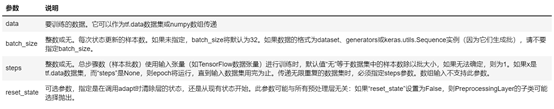
adapt(data, batch_size=None, steps=None, reset_state=True)該函數參數說明如下:
7、構建模型
7.1 構建多層感知器(MLP)
def mlp(x, hidden_units, dropout_rate):for units in hidden_units:x = layers.Dense(units, activation=tf.nn.gelu)(x)x = layers.Dropout(dropout_rate)(x)return x
7.2 創(chuàng)建一個類似卷積層的patch層
class Patches(layers.Layer):def __init__(self, patch_size):super(Patches, self).__init__()self.patch_size = patch_sizedef call(self, images):batch_size = tf.shape(images)[0]patches = tf.image.extract_patches(images=images,sizes=[1, self.patch_size, self.patch_size, 1],strides=[1, self.patch_size, self.patch_size, 1],rates=[1, 1, 1, 1],padding="VALID",)patch_dims = patches.shape[-1]patches = tf.reshape(patches, [batch_size, -1, patch_dims])return patches
7.3 查看由patch層隨機生成的圖像塊
import matplotlib.pyplot as pltplt.figure(figsize=(4, 4))image = x_train[np.random.choice(range(x_train.shape[0]))]plt.imshow(image.astype("uint8"))plt.axis("off")resized_image = tf.image.resize(tf.convert_to_tensor([image]), size=(image_size, image_size))patches = Patches(patch_size)(resized_image)print(f"Image size: {image_size} X {image_size}")print(f"Patch size: {patch_size} X {patch_size}")print(f"Patches per image: {patches.shape[1]}")print(f"Elements per patch: {patches.shape[-1]}")n = int(np.sqrt(patches.shape[1]))plt.figure(figsize=(4, 4))for i, patch in enumerate(patches[0]):ax = plt.subplot(n, n, i + 1)patch_img = tf.reshape(patch, (patch_size, patch_size, 3))plt.imshow(patch_img.numpy().astype("uint8"))plt.axis("off")
運行結果
Image size: 72 X 72
Patch size: 6 X 6
Patches per image: 144
Elements per patch: 108


7.4構建patch 編碼層( encoding layer)
class PatchEncoder(layers.Layer):def __init__(self, num_patches, projection_dim):super(PatchEncoder, self).__init__()self.num_patches = num_patches#一個全連接層,其輸出維度為projection_dim,沒有指明激活函數self.projection = layers.Dense(units=projection_dim)#定義一個嵌入層,這是一個可學習的層#輸入維度為num_patches,輸出維度為projection_dimself.position_embedding = layers.Embedding(input_dim=num_patches, output_dim=projection_dim)def call(self, patch):positions = tf.range(start=0, limit=self.num_patches, delta=1)encoded = self.projection(patch) + self.position_embedding(positions)return encoded
7.5構建ViT模型
def create_vit_classifier():inputs = layers.Input(shape=input_shape)# Augment data.augmented = data_augmentation(inputs)#augmented = augmented_train_batches(inputs)# Create patches.patches = Patches(patch_size)(augmented)# Encode patches.encoded_patches = PatchEncoder(num_patches, projection_dim)(patches)# Create multiple layers of the Transformer block.for _ in range(transformer_layers):# Layer normalization 1.x1 = layers.LayerNormalization(epsilon=1e-6)(encoded_patches)# Create a multi-head attention layer.attention_output = layers.MultiHeadAttention(num_heads=num_heads, key_dim=projection_dim, dropout=0.1x1)# Skip connection 1.x2 = layers.Add()([attention_output, encoded_patches])# Layer normalization 2.x3 = layers.LayerNormalization(epsilon=1e-6)(x2)# MLP.x3 = mlp(x3, hidden_units=transformer_units, dropout_rate=0.1)# Skip connection 2.encoded_patches = layers.Add()([x3, x2])# Create a [batch_size, projection_dim] tensor.representation = layers.LayerNormalization(epsilon=1e-6)(encoded_patches)representation = layers.Flatten()(representation)representation = layers.Dropout(0.5)(representation)# Add MLP.features = mlp(representation, hidden_units=mlp_head_units, dropout_rate=0.5)# Classify outputs.logits = layers.Dense(num_classes)(features)# Create the Keras model.model = keras.Model(inputs=inputs, outputs=logits)return model
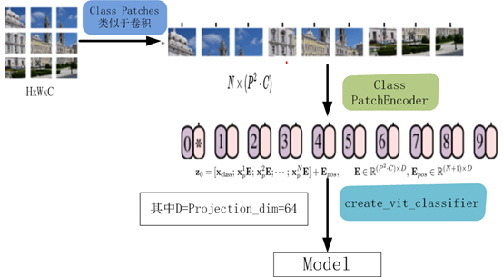
該模型的處理流程如下圖所示
8、編譯、訓練模型
def run_experiment(model):optimizer = tfa.optimizers.AdamW(learning_rate=learning_rate, weight_decay=weight_decay)model.compile(optimizer=optimizer,loss=keras.losses.SparseCategoricalCrossentropy(from_logits=True),metrics=[="accuracy"),name="top-5-accuracy"),],)#checkpoint_filepath = r".\tmp\checkpoint"checkpoint_filepath ="model_bak.hdf5"checkpoint_callback = keras.callbacks.ModelCheckpoint(checkpoint_filepath,monitor="val_accuracy",save_best_only=True,save_weights_only=True,)history = model.fit(x=x_train,y=y_train,batch_size=batch_size,epochs=num_epochs,validation_split=0.1,callbacks=[checkpoint_callback],)model.load_weights(checkpoint_filepath)accuracy, top_5_accuracy = model.evaluate(x_test, y_test)accuracy: {round(accuracy * 100, 2)}%")top 5 accuracy: {round(top_5_accuracy * 100, 2)}%")return history
實例化類,運行模型
vit_classifier = create_vit_classifier()history = run_experiment(vit_classifier)
運行結果
Epoch 1/10
176/176 [==============================] - 68s 333ms/step - loss: 2.6394 - accuracy: 0.2501 - top-5-accuracy: 0.7377 - val_loss: 1.5331 - val_accuracy: 0.4580 - val_top-5-accuracy: 0.9092
Epoch 2/10
176/176 [==============================] - 58s 327ms/step - loss: 1.6359 - accuracy: 0.4150 - top-5-accuracy: 0.8821 - val_loss: 1.2714 - val_accuracy: 0.5348 - val_top-5-accuracy: 0.9464
Epoch 3/10
176/176 [==============================] - 58s 328ms/step - loss: 1.4332 - accuracy: 0.4839 - top-5-accuracy: 0.9210 - val_loss: 1.1633 - val_accuracy: 0.5806 - val_top-5-accuracy: 0.9616
Epoch 4/10
176/176 [==============================] - 58s 329ms/step - loss: 1.3253 - accuracy: 0.5280 - top-5-accuracy: 0.9349 - val_loss: 1.1010 - val_accuracy: 0.6112 - val_top-5-accuracy: 0.9572
Epoch 5/10
176/176 [==============================] - 58s 330ms/step - loss: 1.2380 - accuracy: 0.5626 - top-5-accuracy: 0.9411 - val_loss: 1.0212 - val_accuracy: 0.6400 - val_top-5-accuracy: 0.9690
Epoch 6/10
176/176 [==============================] - 58s 330ms/step - loss: 1.1486 - accuracy: 0.5945 - top-5-accuracy: 0.9520 - val_loss: 0.9698 - val_accuracy: 0.6602 - val_top-5-accuracy: 0.9718
Epoch 7/10
176/176 [==============================] - 58s 330ms/step - loss: 1.1208 - accuracy: 0.6060 - top-5-accuracy: 0.9558 - val_loss: 0.9215 - val_accuracy: 0.6724 - val_top-5-accuracy: 0.9790
Epoch 8/10
176/176 [==============================] - 58s 330ms/step - loss: 1.0643 - accuracy: 0.6248 - top-5-accuracy: 0.9621 - val_loss: 0.8709 - val_accuracy: 0.6944 - val_top-5-accuracy: 0.9768
Epoch 9/10
176/176 [==============================] - 58s 330ms/step - loss: 1.0119 - accuracy: 0.6446 - top-5-accuracy: 0.9640 - val_loss: 0.8290 - val_accuracy: 0.7142 - val_top-5-accuracy: 0.9784
Epoch 10/10
176/176 [==============================] - 58s 330ms/step - loss: 0.9740 - accuracy: 0.6615 - top-5-accuracy: 0.9666 - val_loss: 0.8175 - val_accuracy: 0.7096 - val_top-5-accuracy: 0.9806
313/313 [==============================] - 9s 27ms/step - loss: 0.8514 - accuracy: 0.7032 - top-5-accuracy: 0.9773
Test accuracy: 70.32%
Test top 5 accuracy: 97.73%
In [15]:
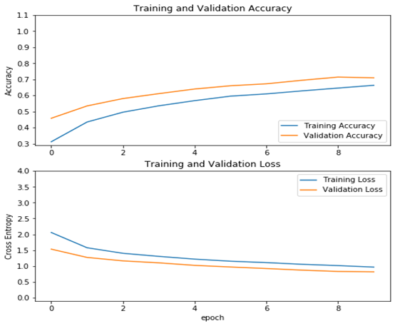
從結果看可以來看,測試精度已達70%,這是一個較大提升!
9、查看運行結果
acc = history.history['accuracy']val_acc = history.history['val_accuracy']loss = history.history['loss']val_loss =history.history['val_loss']plt.figure(figsize=(8, 8))plt.subplot(2, 1, 1)plt.plot(acc, label='Training Accuracy')plt.plot(val_acc, label='Validation Accuracy')plt.legend(loc='lower right')plt.ylabel('Accuracy')plt.ylim([min(plt.ylim()),1.1])plt.title('Training and Validation Accuracy')plt.subplot(2, 1, 2)plt.plot(loss, label='Training Loss')plt.plot(val_loss, label='Validation Loss')plt.legend(loc='upper right')plt.ylabel('Cross Entropy')plt.ylim([-0.1,4.0])plt.title('Training and Validation Loss')plt.xlabel('epoch')plt.show()
運行結果
作者 :吳茂貴,資深大數據和人工智能技術專家,在BI、數據挖掘與分析、數據倉庫、機器學習等領域工作超過20年!在基于Spark、TensorFlow、Pytorch、Keras等機器學習和深度學習方面有大量的工程實踐經驗。代表作有《深入淺出Embedding:原理解析與應用實踐》、《Python深度學習基于Pytorch》和《Python深度學習基于TensorFlow》。
——The End——


點擊購買