↑ 點(diǎn)擊藍(lán)字?關(guān)注極市平臺(tái)

作者丨Gemfield@知乎（已授權(quán)）

來源丨h(huán)ttps://zhuanlan.zhihu.com/p/299108528

編輯丨極市平臺(tái)

極市導(dǎo)讀

本文詳細(xì)介紹了PyTorch對量化的支持的三種方式：模型訓(xùn)練完畢后的動(dòng)態(tài)量化，模型訓(xùn)練完畢后的靜態(tài)量化，模型訓(xùn)練中開啟量化。?>>加入極市CV技術(shù)交流群，走在計(jì)算機(jī)視覺的最前沿

背景

在深度學(xué)習(xí)中，量化指的是使用更少的bit來存儲(chǔ)原本以浮點(diǎn)數(shù)存儲(chǔ)的tensor，以及使用更少的bit來完成原本以浮點(diǎn)數(shù)完成的計(jì)算。這么做的好處主要有如下幾點(diǎn)：

更少的模型體積，接近4倍的減少；
可以更快的計(jì)算，由于更少的內(nèi)存訪問和更快的int8計(jì)算，可以快2~4倍。

一個(gè)量化后的模型，其部分或者全部的tensor操作會(huì)使用int類型來計(jì)算，而不是使用量化之前的float類型。當(dāng)然，量化還需要底層硬件支持，x86 CPU（支持AVX2）、ARM CPU、Google TPU、Nvidia Volta/Turing/Ampere、Qualcomm DSP這些主流硬件都對量化提供了支持。

PyTorch 1.1的時(shí)候開始添加torch.qint8 dtype、torch.quantize_linear轉(zhuǎn)換函數(shù)來開始對量化提供有限的實(shí)驗(yàn)性支持。PyTorch 1.3開始正式支持量化，在可量化的Tensor之外，PyTorch開始支持CNN中最常見的operator的量化操作，包括：

Tensor上的函數(shù): view, clone, resize, slice, add, multiply, cat, mean, max, sort, topk；
常見的模塊（在torch.nn.quantized中）：Conv2d, Linear, Avgpool2d, AdaptiveAvgpool2d, MaxPool2d, AdaptiveMaxPool2d, Interpolate, Upsample；
為了量化后還維持更高準(zhǔn)確率的合并操作（在torch.nn.intrinsic中）：ConvReLU2d, ConvBnReLU2d, ConvBn2d，LinearReLU，add_relu。

在PyTorch 1.4的時(shí)候，PyTorch添加了nn.quantized.Conv3d，與此同時(shí)，torchvision 0.5開始提供量化版本的 ResNet、ResNext、MobileNetV2、GoogleNet、InceptionV3和ShuffleNetV2。到PyTorch 1.5的時(shí)候，QNNPACK添加了對dynamic quantization的支持，也就為量化版的LSTM在手機(jī)平臺(tái)上使用提供了支撐——也就是添加了對PyTorch mobile的dynamic quantization的支持；增加了量化版本的sigmoid、leaky relu、batch_norm、BatchNorm2d、 Avgpool3d、quantized_hardtanh、quantized ELU activation、quantized Upsample3d、quantized batch_norm3d、 batch_norm3d + relu operators的fused、quantized hardsigmoid。

在PyTorch 1.6的時(shí)候，添加了quantized Conv1d、quantized hardswish、quantized layernorm、quantized groupnorm、quantized instancenorm、quantized reflection_pad1d、quantized adaptive avgpool、quantized channel shuffle op、Quantized Threshold；添加ConvBn3d, ConvBnReLU3d, BNReLU2d, BNReLU3d；per-channel的量化得到增強(qiáng)；添加對LSTMCell、RNNCell、GRUCell的Dynamic quantization支持；在nn.DataParallel 和 nn.DistributedDataParallel中可以使用Quantization aware training；支持CUDA上的quantized tensor。

到目前的最新版本的PyTorch 1.7，又添加了Embedding 和EmbeddingBag quantization、aten::repeat、aten::apend、tensor的stack、tensor的fill_、per channel affine quantized tensor的clone、1D batch normalization、N-Dimensional constant padding、CELU operator、FP16 quantization的支持。

PyTorch對量化的支持目前有如下三種方式：

Post Training Dynamic Quantization，模型訓(xùn)練完畢后的動(dòng)態(tài)量化；
Post Training Static Quantization，模型訓(xùn)練完畢后的靜態(tài)量化；
QAT（Quantization Aware Training），模型訓(xùn)練中開啟量化。

在開始這三部分之前，Gemfield先介紹下最基礎(chǔ)的Tensor的量化。

Tensor的量化

PyTorch為了實(shí)現(xiàn)量化，首先就得需要具備能夠表示量化數(shù)據(jù)的Tensor，這就是從PyTorch 1.1之后引入的Quantized Tensor。Quantized Tensor可以存儲(chǔ) int8/uint8/int32類型的數(shù)據(jù)，并攜帶有scale、zero_point這些參數(shù)。把一個(gè)標(biāo)準(zhǔn)的float Tensor轉(zhuǎn)換為量化Tensor的步驟如下：

>>> x = torch.rand(2,3, dtype=torch.float32) >>> xtensor([[0.6839, 0.4741, 0.7451],        [0.9301, 0.1742, 0.6835]])
>>> xq = torch.quantize_per_tensor(x, scale = 0.5, zero_point = 8, dtype=torch.quint8)tensor([[0.5000, 0.5000, 0.5000],        [1.0000, 0.0000, 0.5000]], size=(2, 3), dtype=torch.quint8,       quantization_scheme=torch.per_tensor_affine, scale=0.5, zero_point=8)
>>> xq.int_repr()tensor([[ 9,  9,  9],        [10,  8,  9]], dtype=torch.uint8)

quantize_per_tensor函數(shù)就是使用給定的scale和zp來把一個(gè)float tensor轉(zhuǎn)化為quantized tensor，后文你還會(huì)遇到這個(gè)函數(shù)。通過上面這幾個(gè)數(shù)的變化，你可以感受到，量化tensor，也就是xq，和fp32 tensor的關(guān)系大概就是:

xq = round(x / scale + zero_point)

scale這個(gè)縮放因子和zero_point是兩個(gè)參數(shù)，建立起了fp32 tensor到量化tensor的映射關(guān)系。scale體現(xiàn)了映射中的比例關(guān)系，而zero_point則是零基準(zhǔn)，也就是fp32中的零在量化tensor中的值。因?yàn)楫?dāng)x為零的時(shí)候，上述xq就變成了：

xq = round(zero_point) = zero_point

現(xiàn)在xq已經(jīng)是一個(gè)量化tensor了，我們可以把xq在反量化回來，如下所示：

# xq is a quantized tensor with data represented as quint8>>> xdq = xq.dequantize()>>> xdqtensor([[0.5000, 0.5000, 0.5000],        [1.0000, 0.0000, 0.5000]])

dequantize函數(shù)就是quantize_per_tensor的反義詞，把一個(gè)量化tensor轉(zhuǎn)換為float tensor。也就是：

xdq = (xq - zero_point) * scale

xdq和x的值已經(jīng)出現(xiàn)了偏差的事實(shí)告訴了我們兩個(gè)道理：

量化會(huì)有精度損失；
我們這里隨便選取的scale和zp太爛，選擇合適的scale和zp可以有效降低精度損失。不信你把scale和zp分別換成scale = 0.0036, zero_point = 0試試。

而在PyTorch中，選擇合適的scale和zp的工作就由各種observer來完成。

Tensor的量化支持兩種模式：per tensor 和 per channel。Per tensor 是說一個(gè)tensor里的所有value按照同一種方式去scale和offset；per channel是對于tensor的某一個(gè)維度（通常是channel的維度）上的值按照一種方式去scale和offset，也就是一個(gè)tensor里有多種不同的scale和offset的方式（組成一個(gè)vector），如此以來，在量化的時(shí)候相比per tensor的方式會(huì)引入更少的錯(cuò)誤。PyTorch目前支持conv2d()、conv3d()、linear()的per channel量化。

Post Training Dynamic Quantization

這種量化方式經(jīng)常縮略前面的兩個(gè)單詞從而稱之為Dynamic Quantization，中文為動(dòng)態(tài)量化。這是什么意思呢？你看到全稱中的兩個(gè)關(guān)鍵字了嗎：Post、Dynamic：

Post：也就是訓(xùn)練完成后再量化模型的權(quán)重參數(shù)；
Dynamic：也就是網(wǎng)絡(luò)在前向推理的時(shí)候動(dòng)態(tài)的量化float32類型的輸入。

Dynamic Quantization使用下面的API來完成模型的量化：

torch.quantization.quantize_dynamic(model, qconfig_spec=None, dtype=torch.qint8, mapping=None, inplace=False)

quantize_dynamic這個(gè)API把一個(gè)float model轉(zhuǎn)換為dynamic quantized model，也就是只有權(quán)重被量化的model，dtype參數(shù)可以取值 float16 或者 qint8。當(dāng)對整個(gè)模型進(jìn)行轉(zhuǎn)換時(shí)，默認(rèn)只對以下的op進(jìn)行轉(zhuǎn)換：

Linear
LSTM
LSTMCell
RNNCell
GRUCell

為啥呢？因?yàn)閐ynamic quantization只是把權(quán)重參數(shù)進(jìn)行量化，而這些layer一般參數(shù)數(shù)量很大，在整個(gè)模型中參數(shù)量占比極高，因此邊際效益高。對其它layer進(jìn)行dynamic quantization幾乎沒有實(shí)際的意義。

再來說說這個(gè)API的第二個(gè)參數(shù)：qconfig_spec：

qconfig_spec指定了一組qconfig，具體就是哪個(gè)op對應(yīng)哪個(gè)qconfig ；
每個(gè)qconfig是QConfig類的實(shí)例，封裝了兩個(gè)observer；
這兩個(gè)observer分別是activation的observer和weight的observer；
但是動(dòng)態(tài)量化使用的是QConfig子類QConfigDynamic的實(shí)例，該實(shí)例實(shí)際上只封裝了weight的observer；
activate就是post process，就是op forward之后的后處理，但在動(dòng)態(tài)量化中不包含；
observer用來根據(jù)四元組（min_val，max_val，qmin, qmax）來計(jì)算2個(gè)量化的參數(shù)：scale和zero_point；
qmin、qmax是算法提前確定好的，min_val和max_val是從輸入數(shù)據(jù)中觀察到的，所以起名叫observer。

當(dāng)qconfig_spec為None的時(shí)候就是默認(rèn)行為，如果想要改變默認(rèn)行為，則可以：

qconfig_spec賦值為一個(gè)set，比如：{nn.LSTM, nn.Linear}，意思是指定當(dāng)前模型中的哪些layer要被dynamic quantization；
qconfig_spec賦值為一個(gè)dict，key為submodule的name或type，value為QConfigDynamic實(shí)例（其包含了特定的Observer，比如MinMaxObserver、MovingAverageMinMaxObserver、PerChannelMinMaxObserver、MovingAveragePerChannelMinMaxObserver、HistogramObserver）。

事實(shí)上，當(dāng)qconfig_spec為None的時(shí)候，quantize_dynamic API就會(huì)使用如下的默認(rèn)值：

 qconfig_spec = {                nn.Linear : default_dynamic_qconfig,                nn.LSTM : default_dynamic_qconfig,                nn.GRU : default_dynamic_qconfig,                nn.LSTMCell : default_dynamic_qconfig,                nn.RNNCell : default_dynamic_qconfig,                nn.GRUCell : default_dynamic_qconfig,            }

這就是Gemfield剛才提到的動(dòng)態(tài)量化只量化Linear和RNN變種的真相。而default_dynamic_qconfig是QConfigDynamic的一個(gè)實(shí)例，使用如下的參數(shù)進(jìn)行構(gòu)造：

default_dynamic_qconfig = QConfigDynamic(activation=default_dynamic_quant_observer, weight=default_weight_observer)default_dynamic_quant_observer = PlaceholderObserver.with_args(dtype=torch.float, compute_dtype=torch.quint8)default_weight_observer = MinMaxObserver.with_args(dtype=torch.qint8, qscheme=torch.per_tensor_symmetric)

其中，用于activation的PlaceholderObserver 就是個(gè)占位符，啥也不做；而用于weight的MinMaxObserver就是記錄輸入tensor中的最大值和最小值，用來計(jì)算scale和zp。

對于一個(gè)默認(rèn)行為下的quantize_dynamic調(diào)用，你的模型會(huì)經(jīng)歷什么變化呢？Gemfield使用一個(gè)小網(wǎng)絡(luò)來演示下：

class CivilNet(nn.Module):    def __init__(self):        super(CivilNet, self).__init__()        gemfieldin = 1        gemfieldout = 1        self.conv = nn.Conv2d(gemfieldin, gemfieldout, kernel_size=1, stride=1, padding=0, groups=1, bias=False)        self.fc = nn.Linear(3, 2,bias=False)        self.relu = nn.ReLU(inplace=False)
    def forward(self, x):        x = self.conv(x)        x = self.fc(x)        x = self.relu(x)        return x

原始網(wǎng)絡(luò)和動(dòng)態(tài)量化后的網(wǎng)絡(luò)如下所示：

#原始網(wǎng)絡(luò)CivilNet(  (conv): Conv2d(1, 1, kernel_size=(1, 1), stride=(1, 1), bias=False)  (fc): Linear(in_features=3, out_features=2, bias=False)  (relu): ReLU())
#quantize_dynamic 后CivilNet(  (conv): Conv2d(1, 1, kernel_size=(1, 1), stride=(1, 1), bias=False)  (fc): DynamicQuantizedLinear(in_features=3, out_features=2, dtype=torch.qint8, qscheme=torch.per_tensor_affine)  (relu): ReLU())

可以看到，除了Linear，其它op都沒有變動(dòng)。而Linear被轉(zhuǎn)換成了DynamicQuantizedLinear，DynamicQuantizedLinear就是torch.nn.quantized.dynamic.modules.linear.Linear類。沒錯(cuò)，quantize_dynamic API的本質(zhì)就是檢索模型中op的type，如果某個(gè)op的type屬于字典DEFAULT_DYNAMIC_QUANT_MODULE_MAPPINGS的key，那么，這個(gè)op將被替換為key對應(yīng)的value：

# Default map for swapping dynamic modulesDEFAULT_DYNAMIC_QUANT_MODULE_MAPPINGS = {    nn.GRUCell: nnqd.GRUCell,    nn.Linear: nnqd.Linear,    nn.LSTM: nnqd.LSTM,    nn.LSTMCell: nnqd.LSTMCell,    nn.RNNCell: nnqd.RNNCell,}

這里，nnqd.Linear就是DynamicQuantizedLinear就是torch.nn.quantized.dynamic.modules.linear.Linear。但是，type從key換為value，那這個(gè)新的type如何實(shí)例化呢？更重要的是，實(shí)例化新的type一定是要用之前的權(quán)重參數(shù)的呀。沒錯(cuò)，以Linear為例，該邏輯定義在 nnqd.Linear的from_float()方法中，通過如下方式實(shí)例化：

new_mod = mapping[type(mod)].from_float(mod)

from_float做的事情主要就是：

使用MinMaxObserver計(jì)算模型中op權(quán)重參數(shù)中tensor的最大值最小值（這個(gè)例子中只有Linear op），縮小量化時(shí)原始值的取值范圍，提高量化的精度；
通過上述步驟中得到四元組中的min_val和max_val，再結(jié)合算法確定的qmin, qmax計(jì)算出scale和zp，參考前文“Tensor的量化”小節(jié)，計(jì)算得到量化后的weight，這個(gè)量化過程有torch.quantize_per_tensor和torch.quantize_per_channel兩種，默認(rèn)是前者（因?yàn)閝chema默認(rèn)是torch.per_tensor_affine）；
實(shí)例化nnqd.Linear，然后使用qlinear.set_weight_bias將量化后的weight和原始的bias設(shè)置到新的layer上。其中最后一步還涉及到weight和bias的打包，在源代碼中是這樣的：

#ifdef USE_FBGEMM    if (ctx.qEngine() == at::QEngine::FBGEMM) {      return PackedLinearWeight::prepack(std::move(weight), std::move(bias));    }#endif
#ifdef USE_PYTORCH_QNNPACK    if (ctx.qEngine() == at::QEngine::QNNPACK) {      return PackedLinearWeightsQnnp::prepack(std::move(weight), std::move(bias));    }#endif    TORCH_CHECK(false,"Didn't find engine for operation quantized::linear_prepack ",toString(ctx.qEngine()));

也就是說依賴FBGEMM、QNNPACK這些backend。量化完后的模型在推理的時(shí)候有什么不一樣的呢？在原始網(wǎng)絡(luò)中，從輸入到最終輸出是這么計(jì)算的：

#inputtorch.Tensor([[[[-1,-2,-3],[1,2,3]]]])
#經(jīng)過卷積后（權(quán)重為torch.Tensor([[[[-0.7867]]]])）torch.Tensor([[[[ 0.7867,  1.5734,  2.3601],[-0.7867, -1.5734, -2.3601]]]])
#經(jīng)過fc后（權(quán)重為torch.Tensor([[ 0.4097, -0.2896, -0.4931], [-0.3738, -0.5541,  0.3243]]) )torch.Tensor([[[[-1.2972, -0.4004], [1.2972,  0.4004]]]])
#經(jīng)過relu后torch.Tensor([[[[0.0000, 0.0000],[1.2972, 0.4004]]]])

而在動(dòng)態(tài)量化模型中，上述過程就變成了：

#inputtorch.Tensor([[[[-1,-2,-3],[1,2,3]]]])
#經(jīng)過卷積后（權(quán)重為torch.Tensor([[[[-0.7867]]]])）torch.Tensor([[[[ 0.7867,  1.5734,  2.3601],[-0.7867, -1.5734, -2.3601]]]])
#經(jīng)過fc后（權(quán)重為torch.Tensor([[ 0.4085, -0.2912, -0.4911],[-0.3737, -0.5563,  0.3259]], dtype=torch.qint8,scale=0.0043458822183310986,zero_point=0) )torch.Tensor([[[[-1.3038, -0.3847], [1.2856,  0.3969]]]])
#經(jīng)過relu后torch.Tensor([[[[0.0000, 0.0000], [1.2856, 0.3969]]]])

所以關(guān)鍵點(diǎn)就是這里的Linear op了，因?yàn)槠渌黲p和量化之前是一模一樣的。你可以看到Linear權(quán)重的scale為0.0043458822183310986，zero_point為0。scale和zero_point怎么來的呢？由其使用的observer計(jì)算得到的，具體來說就是默認(rèn)的MinMaxObserver，它是怎么工作的呢？還記得前面說過的observer負(fù)責(zé)根據(jù)四元組來計(jì)算scale和zp吧：

在各種observer中，計(jì)算權(quán)重的scale和zp離不開這四個(gè)變量：min_val，max_val，qmin, qmax，分別代表op權(quán)重?cái)?shù)據(jù)/input tensor數(shù)據(jù)分布的最小值和最大值，以及量化后的取值范圍的最小、最大值。qmin和qmax的值好確定，基本就是8個(gè)bit能表示的范圍，這里取的分別是-128和127（更詳細(xì)的計(jì)算方式將會(huì)在下文的“靜態(tài)量化”章節(jié)中描述）；Linear op的權(quán)重為torch.Tensor([[ 0.4097, -0.2896, -0.4931], [-0.3738, -0.5541, 0.3243]])，因此其min_val和max_val分別為-0.5541 和 0.4097，在這個(gè)上下文中，max_val將進(jìn)一步取這倆絕對值的最大值。由此我們就可以得到：

scale = max_val / (float(qmax - qmin) / 2) = 0.5541 / ((127 + 128) / 2) = 0.004345882...
zp = 0

scale和zp的計(jì)算細(xì)節(jié)還會(huì)在下文的“靜態(tài)量化”章節(jié)中更詳細(xì)的描述。從上面我們可以得知，權(quán)重部分的量化是“靜態(tài)”的，是提前就轉(zhuǎn)換完畢的，而之所以叫做“動(dòng)態(tài)”量化，就在于前向推理的時(shí)候動(dòng)態(tài)的把input的float tensor轉(zhuǎn)換為量化tensor。

在forward的時(shí)候，nnqd.Linear會(huì)調(diào)用torch.ops.quantized.linear_dynamic函數(shù)，輸入正是上面（pack好后的）量化后的權(quán)重和float的bias，而torch.ops.quantized.linear_dynamic函數(shù)最終會(huì)被PyTorch分發(fā)到C++中的apply_dynamic_impl函數(shù)，在這里，或者使用FBGEMM的實(shí)現(xiàn)（x86-64設(shè)備），或者使用QNNPACK的實(shí)現(xiàn)（ARM設(shè)備上）：

#ifdef USE_FBGEMMat::Tensor PackedLinearWeight::apply_dynamic_impl(at::Tensor input, bool reduce_range) {  ...  fbgemm::xxxx  ...}#endif // USE_FBGEMM
#ifdef USE_PYTORCH_QNNPACKat::Tensor PackedLinearWeightsQnnp::apply_dynamic_impl(at::Tensor input) {  ...  qnnpack::qnnpackLinearDynamic(xxxx)  ...}#endif // USE_PYTORCH_QNNPACK

等等，input還是float32的啊，這怎么運(yùn)算嘛。別急，在上述的apply_dynamic_impl函數(shù)中，會(huì)使用下面的邏輯對輸入進(jìn)行量化：

Tensor q_input = at::quantize_per_tensor(input_contig, q_params.scale, q_params.zero_point, c10::kQUInt8);

也就是說，動(dòng)態(tài)量化的本質(zhì)就藏身于此：基于運(yùn)行時(shí)對數(shù)據(jù)范圍的觀察，來動(dòng)態(tài)確定對輸入進(jìn)行量化時(shí)的scale值。這就確保 input tensor的scale因子能夠基于輸入數(shù)據(jù)進(jìn)行優(yōu)化，從而獲得顆粒度更細(xì)的信息。

而模型的參數(shù)則是提前就轉(zhuǎn)換為了INT8的格式（在使用quantize_dynamic API的時(shí)候）。這樣，當(dāng)輸入也被量化后，網(wǎng)絡(luò)中的運(yùn)算就使用向量化的INT8指令來完成。而在當(dāng)前l(fā)ayer輸出的時(shí)候，我們還需要把結(jié)果再重新轉(zhuǎn)換為float32——re-quantization的scale值是依據(jù)input、 weight和output scale來確定的，定義如下：
requant_scale = input_scale_fp32 * weight_scale_fp32 / output_scale_fp32

實(shí)際上，在apply_dynamic_impl函數(shù)中，requant_scales就是這么實(shí)現(xiàn)的：

auto output_scale = 1.fauto inverse_output_scale = 1.f /output_scale;requant_scales[i] = (weight_scales_data[i] * input_scale) * inverse_output_scale;

這就是為什么在前面Gemfield提到過，經(jīng)過量化版的fc的輸出為torch.Tensor([[[[-1.3038, -0.3847], [1.2856, 0.3969]]]])，已經(jīng)變回正常的float tensor了。所以動(dòng)態(tài)量化模型的前向推理過程可以概括如下：

#原始的模型，所有的tensor和計(jì)算都是浮點(diǎn)型previous_layer_fp32 -- linear_fp32 -- activation_fp32 -- next_layer_fp32                 /linear_weight_fp32
#動(dòng)態(tài)量化后的模型，Linear和LSTM的權(quán)重是int8previous_layer_fp32 -- linear_int8_w_fp32_inp -- activation_fp32 -- next_layer_fp32                     /   linear_weight_int8

總結(jié)下來，我們可以這么說：Post Training Dynamic Quantization，簡稱為Dynamic Quantization，也就是動(dòng)態(tài)量化，或者叫作Weight-only的量化，是提前把模型中某些op的參數(shù)量化為INT8，然后在運(yùn)行的時(shí)候動(dòng)態(tài)的把輸入量化為INT8，然后在當(dāng)前op輸出的時(shí)候再把結(jié)果requantization回到float32類型。動(dòng)態(tài)量化默認(rèn)只適用于Linear以及RNN的變種。

Post Training Static Quantization

與其介紹post training static quantization是什么，我們不如先來說明下它和dynamic quantization的相同點(diǎn)和區(qū)別是什么。相同點(diǎn)就是，都是把網(wǎng)絡(luò)的權(quán)重參數(shù)轉(zhuǎn)從float32轉(zhuǎn)換為int8；不同點(diǎn)是，需要把訓(xùn)練集或者和訓(xùn)練集分布類似的數(shù)據(jù)喂給模型（注意沒有反向傳播），然后通過每個(gè)op輸入的分布特點(diǎn)來計(jì)算activation的量化參數(shù)（scale和zp）——稱之為Calibrate（定標(biāo)）。是的，靜態(tài)量化包含有activation了，也就是post process，也就是op forward之后的后處理。為什么靜態(tài)量化需要activation呢？因?yàn)殪o態(tài)量化的前向推理過程自(始+1)至(終-1)都是INT計(jì)算，activation需要確保一個(gè)op的輸入符合下一個(gè)op的輸入。

PyTorch會(huì)使用五部曲來完成模型的靜態(tài)量化：

1，fuse_model

合并一些可以合并的layer。這一步的目的是為了提高速度和準(zhǔn)確度：

fuse_modules(model, modules_to_fuse, inplace=False, fuser_func=fuse_known_modules, fuse_custom_config_dict=None)

比如給fuse_modules傳遞下面的參數(shù)就會(huì)合并網(wǎng)絡(luò)中的conv1、bn1、relu1：

torch.quantization.fuse_modules(gemfield_model, [['conv1', 'bn1', 'relu1']], inplace=True)

一旦合并成功，那么原始網(wǎng)絡(luò)中的conv1就會(huì)被替換為新的合并后的module（因?yàn)槠涫莑ist中的第一個(gè)元素），而bn1、relu1（list中剩余的元素）會(huì)被替換為nn.Identity()，這個(gè)模塊是個(gè)占位符，直接輸出輸入。舉個(gè)例子，對于下面的一個(gè)小網(wǎng)絡(luò)：

class CivilNet(nn.Module):    def __init__(self):        super(CivilNet, self).__init__()        syszuxin = 1        syszuxout = 1        self.conv = nn.Conv2d(syszuxin, syszuxout, kernel_size=1, stride=1, padding=0, groups=1, bias=False)        self.fc = nn.Linear(3, 2,bias=False)        self.relu = nn.ReLU(inplace=False)
    def forward(self, x):        x = self.conv(x)        x = self.fc(x)        x = self.relu(x)        return x

網(wǎng)絡(luò)結(jié)構(gòu)如下：

CivilNet(  (conv): Conv2d(1, 1, kernel_size=(1, 1), stride=(1, 1), bias=False)  (fc): Linear(in_features=3, out_features=2, bias=False)  (relu): ReLU())

經(jīng)過torch.quantization.fuse_modules(c, [['fc',?'relu']], inplace=True)后，網(wǎng)絡(luò)變成了：

CivilNet(  (conv): Conv2d(1, 1, kernel_size=(1, 1), stride=(1, 1), bias=False)  (fc): LinearReLU(    (0): Linear(in_features=3, out_features=2, bias=False)    (1): ReLU()  )  (relu): Identity())

modules_to_fuse參數(shù)的list可以包含多個(gè)item list，或者是submodule的op list也可以，比如：[ ['conv1', 'bn1', 'relu1'], ['submodule.conv', 'submodule.relu']]。有的人會(huì)說了，我要fuse的module被Sequential封裝起來了，如何傳參？參考下面的代碼：

torch.quantization.fuse_modules(a_sequential_module, ['0', '1', '2'], inplace=True)

不是什么類型的op都可以參與合并，也不是什么樣的順序都可以參與合并。就目前來說，截止到pytorch 1.7.1，只有如下的op和順序才可以：

Convolution, Batch normalization
Convolution, Batch normalization, Relu
Convolution, Relu
Linear, Relu
Batch normalization, Relu

實(shí)際上，這個(gè)mapping關(guān)系就定義在DEFAULT_OP_LIST_TO_FUSER_METHOD中：

DEFAULT_OP_LIST_TO_FUSER_METHOD : Dict[Tuple, Union[nn.Sequential, Callable]] = {    (nn.Conv1d, nn.BatchNorm1d): fuse_conv_bn,    (nn.Conv1d, nn.BatchNorm1d, nn.ReLU): fuse_conv_bn_relu,    (nn.Conv2d, nn.BatchNorm2d): fuse_conv_bn,    (nn.Conv2d, nn.BatchNorm2d, nn.ReLU): fuse_conv_bn_relu,    (nn.Conv3d, nn.BatchNorm3d): fuse_conv_bn,    (nn.Conv3d, nn.BatchNorm3d, nn.ReLU): fuse_conv_bn_relu,    (nn.Conv1d, nn.ReLU): nni.ConvReLU1d,    (nn.Conv2d, nn.ReLU): nni.ConvReLU2d,    (nn.Conv3d, nn.ReLU): nni.ConvReLU3d,    (nn.Linear, nn.ReLU): nni.LinearReLU,    (nn.BatchNorm2d, nn.ReLU): nni.BNReLU2d,    (nn.BatchNorm3d, nn.ReLU): nni.BNReLU3d,}

2，設(shè)置qconfig

qconfig是要設(shè)置到模型或者模型的子module上的。前文Gemfield就已經(jīng)說過，qconfig是QConfig的一個(gè)實(shí)例，QConfig這個(gè)類就是維護(hù)了兩個(gè)observer，一個(gè)是activation所使用的observer，一個(gè)是op權(quán)重所使用的observer。

#如果要部署在x86 server上gemfield_model.qconfig = torch.quantization.get_default_qconfig('fbgemm')
#如果要部署在ARM上gemfield_model.qconfig = torch.quantization.get_default_qconfig('qnnpack')

如果是x86和arm之外呢？抱歉，目前不支持。實(shí)際上，這里的get_default_qconfig函數(shù)的實(shí)現(xiàn)如下所示：

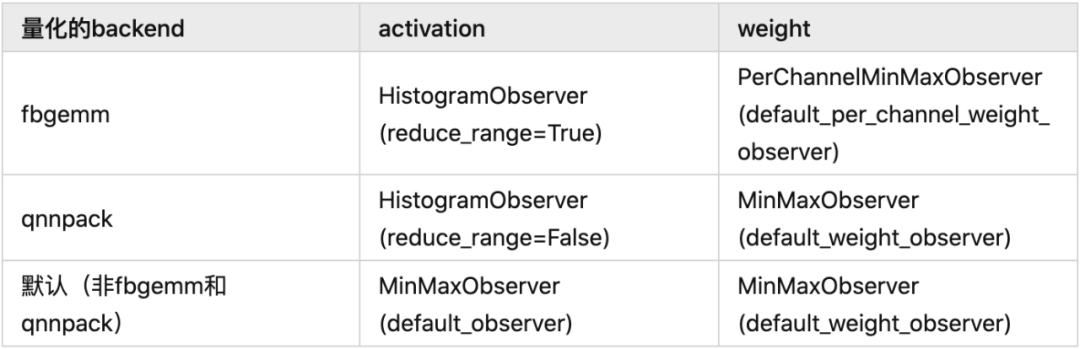
def get_default_qconfig(backend='fbgemm'):    if backend == 'fbgemm':        qconfig = QConfig(activation=HistogramObserver.with_args(reduce_range=True),weight=default_per_channel_weight_observer)    elif backend == 'qnnpack':        qconfig = QConfig(activation=HistogramObserver.with_args(reduce_range=False),weight=default_weight_observer)    else:        qconfig = default_qconfig    return qconfig

default_qconfig實(shí)際上是QConfig(activation=default_observer, weight=default_weight_observer)，所以gemfield這里總結(jié)了一個(gè)表格：

3，prepare

prepare調(diào)用是通過如下API完成的：

gemfield_model_prepared = torch.quantization.prepare(gemfield_model)

prepare用來給每個(gè)子module插入Observer，用來收集和定標(biāo)數(shù)據(jù)。以activation的observer為例，就是期望其觀察輸入數(shù)據(jù)得到四元組中的min_val和max_val，至少觀察個(gè)幾百個(gè)迭代的數(shù)據(jù)吧，然后由這四元組得到scale和zp這兩個(gè)參數(shù)的值。

module上安插activation的observer是怎么實(shí)現(xiàn)的呢？還記得zhuanlan.zhihu.com/p/53一文中說過的“_forward_hooks是通過register_forward_hook來完成注冊的。這些hooks是在forward完之后被調(diào)用的......”嗎？沒錯(cuò)，CivilNet模型中的Conv2d、Linear、ReLU、QuantStub這些module的_forward_hooks上都被插入了activation的HistogramObserver，當(dāng)這些子module計(jì)算完畢后，結(jié)果會(huì)被立刻送到其_forward_hooks中的HistogramObserver進(jìn)行觀察。

這一步完成后，CivilNet網(wǎng)絡(luò)就被改造成了：

CivilNet(  (conv): Conv2d(    1, 1, kernel_size=(1, 1), stride=(1, 1), bias=False    (activation_post_process): HistogramObserver()  )  (fc): Linear(    in_features=3, out_features=2, bias=False    (activation_post_process): HistogramObserver()  )  (relu): ReLU(    (activation_post_process): HistogramObserver()  )  (quant): QuantStub(    (activation_post_process): HistogramObserver()  )  (dequant): DeQuantStub())

4，喂數(shù)據(jù)

這一步不是訓(xùn)練。是為了獲取數(shù)據(jù)的分布特點(diǎn)，來更好的計(jì)算activation的scale和zp。至少要喂上幾百個(gè)迭代的數(shù)據(jù)。

#至少觀察個(gè)幾百迭代for data in data_loader:    gemfield_model_prepared(data)

5，轉(zhuǎn)換模型

第四步完成后，各個(gè)op權(quán)重的四元組（min_val，max_val，qmin, qmax）中的min_val，max_val已經(jīng)有了，各個(gè)op activation的四元組（min_val，max_val，qmin, qmax）中的min_val，max_val也已經(jīng)觀察出來了。那么在這一步我們將調(diào)用convert API：

gemfield_model_prepared_int8 = torch.quantization.convert(gemfield_model_prepared)

這個(gè)過程和dynamic量化類似，本質(zhì)就是檢索模型中op的type，如果某個(gè)op的type屬于字典DEFAULT_STATIC_QUANT_MODULE_MAPPINGS的key（注意字典和動(dòng)態(tài)量化的不一樣了），那么，這個(gè)op將被替換為key對應(yīng)的value：

DEFAULT_STATIC_QUANT_MODULE_MAPPINGS = {    QuantStub: nnq.Quantize,    DeQuantStub: nnq.DeQuantize,    nn.BatchNorm2d: nnq.BatchNorm2d,    nn.BatchNorm3d: nnq.BatchNorm3d,    nn.Conv1d: nnq.Conv1d,    nn.Conv2d: nnq.Conv2d,    nn.Conv3d: nnq.Conv3d,    nn.ConvTranspose1d: nnq.ConvTranspose1d,    nn.ConvTranspose2d: nnq.ConvTranspose2d,    nn.ELU: nnq.ELU,    nn.Embedding: nnq.Embedding,    nn.EmbeddingBag: nnq.EmbeddingBag,    nn.GroupNorm: nnq.GroupNorm,    nn.Hardswish: nnq.Hardswish,    nn.InstanceNorm1d: nnq.InstanceNorm1d,    nn.InstanceNorm2d: nnq.InstanceNorm2d,    nn.InstanceNorm3d: nnq.InstanceNorm3d,    nn.LayerNorm: nnq.LayerNorm,    nn.LeakyReLU: nnq.LeakyReLU,    nn.Linear: nnq.Linear,    nn.ReLU6: nnq.ReLU6,    # Wrapper Modules:    nnq.FloatFunctional: nnq.QFunctional,    # Intrinsic modules:    nni.BNReLU2d: nniq.BNReLU2d,    nni.BNReLU3d: nniq.BNReLU3d,    nni.ConvReLU1d: nniq.ConvReLU1d,    nni.ConvReLU2d: nniq.ConvReLU2d,    nni.ConvReLU3d: nniq.ConvReLU3d,    nni.LinearReLU: nniq.LinearReLU,    nniqat.ConvBn1d: nnq.Conv1d,    nniqat.ConvBn2d: nnq.Conv2d,    nniqat.ConvBnReLU1d: nniq.ConvReLU1d,    nniqat.ConvBnReLU2d: nniq.ConvReLU2d,    nniqat.ConvReLU2d: nniq.ConvReLU2d,    nniqat.LinearReLU: nniq.LinearReLU,    # QAT modules:    nnqat.Linear: nnq.Linear,    nnqat.Conv2d: nnq.Conv2d,}

替換的過程也和dynamic一樣，使用from_float() API，這個(gè)API會(huì)使用前面的四元組信息計(jì)算出op權(quán)重和op activation的scale和zp，然后用于量化。動(dòng)態(tài)量化”章節(jié)時(shí)Gemfield說過要再詳細(xì)介紹下scale和zp的計(jì)算過程，好了，就在這里。這個(gè)計(jì)算過程覆蓋了如下的幾個(gè)問題：

QuantStub的scale和zp是怎么來的（靜態(tài)量化需要插入QuantStub，后文有說明）？
conv activation的scale和zp是怎么來的？
conv weight的scale和zp是怎么來的？
fc activation的scale和zp是怎么來的？
fc weight的scale和zp是怎么來的？
relu activation的scale和zp是怎么來的？
relu weight的...等等，relu沒有weight。

我們就從conv來說起吧，還記得前面說過的Observer嗎？分為activation和weight兩種。以Gemfield這里使用的fbgemm后端為例，activation默認(rèn)的observer是HistogramObserver、weight默認(rèn)的observer是PerChannelMinMaxObserver。而計(jì)算scale和zp所需的四元組都是這些observer觀察出來的呀（好吧，其中兩個(gè)）。

在convert API調(diào)用中，pytorch會(huì)將Conv2d op替換為對應(yīng)的QuantizedConv2d，在這個(gè)替換的過程中會(huì)計(jì)算QuantizedConv2d activation的scale和zp以及QuantizedConv2d weight的scale和zp。在各種observer中，計(jì)算scale和zp離不開這四個(gè)變量：min_val，max_val，qmin, qmax，分別代表輸入的數(shù)據(jù)/權(quán)重的數(shù)據(jù)分布的最小值和最大值，以及量化后的取值范圍的最小、最大值。qmin和qmax的值好確定，基本就是8個(gè)bit能表示的范圍，在pytorch中，qmin和qmax是使用如下方式確定的：

if self.dtype == torch.qint8:    if self.reduce_range:        qmin, qmax = -64, 63    else:        qmin, qmax = -128, 127else:    if self.reduce_range:        qmin, qmax = 0, 127    else:        qmin, qmax = 0, 255

比如conv的activation的observer(quint8)是HistogramObserver，又是reduce_range的，因此其qmin,qmax = 0 ，127，而conv的weight(qint8)是PerChannelMinMaxObserver，不是reduce_range的，因此其qmin, qmax = -128, 127。那么min_val，max_val又是怎么確定的呢？對于HistogramObserver，其由輸入數(shù)據(jù) + 權(quán)重值根據(jù)L2Norm(An approximation for L2 error minimization)確定；對于PerChannelMinMaxObserver來說，其由輸入數(shù)據(jù)的最小值和最大值確定，比如在上述的例子中，值就是-0.7898和-0.7898。既然現(xiàn)在conv weight的min_val，max_val，qmin, qmax 分別為 -0.7898、-0.7898、-128、 127，那如何得到scale和zp呢？PyTorch就是用下面的邏輯進(jìn)行計(jì)算的：

#qscheme 是 torch.per_tensor_symmetric 或者torch.per_channel_symmetric時(shí)max_val = torch.max(-min_val, max_val)scale = max_val / (float(qmax - qmin) / 2)scale = torch.max(scale, torch.tensor(self.eps, device=device, dtype=scale.dtype))if self.dtype == torch.quint8:    zero_point = zero_point.new_full(zero_point.size(), 128)
#qscheme 是 torch.per_tensor_affine時(shí)scale = (max_val - min_val) / float(qmax - qmin)scale = torch.max(scale, torch.tensor(self.eps, device=device, dtype=scale.dtype))zero_point = qmin - torch.round(min_val / scale)zero_point = torch.max(zero_point, torch.tensor(qmin, device=device, dtype=zero_point.dtype))zero_point = torch.min(zero_point, torch.tensor(qmax, device=device, dtype=zero_point.dtype))

由此conv2d weight的謎團(tuán)就被我們解開了：

scale = 0.7898 / ((127 + 128)/2 ) = 0.0062
zp = 0

再說說QuantStub的scale和zp是如何計(jì)算的。QuantStub使用的是HistogramObserver，根據(jù)輸入從[-3,3]的分布，HistogramObserver計(jì)算得到min_val、max_val分別是-3、2.9971，而qmin和qmax又分別是0、127，其schema為per_tensor_affine，因此套用上面的per_tensor_affine邏輯可得：

scale = (2.9971 + 3) / (127 - 0) = 0.0472
zp = 0 - round(-3 /0.0472) = 64

其它計(jì)算同理，不再贅述。有了scale和zp，就有了量化版本的module，上面那個(gè)CivilNet網(wǎng)絡(luò)，經(jīng)過靜態(tài)量化后，網(wǎng)絡(luò)的變化如下所示：

#原始的CivilNet網(wǎng)絡(luò)：CivilNet(  (conv): Conv2d(1, 1, kernel_size=(1, 1), stride=(1, 1), bias=False)  (fc): Linear(in_features=3, out_features=2, bias=False)  (relu): ReLU())
#靜態(tài)量化后的CivilNet網(wǎng)絡(luò)：CivilNet(  (conv): QuantizedConv2d(1, 1, kernel_size=(1, 1), stride=(1, 1), scale=0.0077941399067640305, zero_point=0, bias=False)  (fc): QuantizedLinear(in_features=3, out_features=2, scale=0.002811126410961151, zero_point=14, qscheme=torch.per_channel_affine)  (relu): QuantizedReLU())

靜態(tài)量化模型如何推理？

我們知道，在PyTorch的網(wǎng)絡(luò)中，前向推理邏輯都是實(shí)現(xiàn)在了每個(gè)op的forward函數(shù)中（參考：Gemfield：詳解Pytorch中的網(wǎng)絡(luò)構(gòu)造）（https://zhuanlan.zhihu.com/p/53927068）。而在convert完成后，所有的op被替換成了量化版本的op，那么量化版本的op的forward會(huì)有什么不一樣的呢？還記得嗎？動(dòng)態(tài)量化中可是只量化了op的權(quán)重哦，輸入的量化所需的scale的值是在推理過程中動(dòng)態(tài)計(jì)算出來的。而靜態(tài)量化中，統(tǒng)統(tǒng)都是提前就計(jì)算好的。我們來看一個(gè)典型的靜態(tài)量化模型的推理過程：

import torchimport torch.nn as nn
class CivilNet(nn.Module):    def __init__(self):        super(CivilNet, self).__init__()        in_planes = 1        out_planes = 1        self.conv = nn.Conv2d(in_planes, out_planes, kernel_size=1, stride=1, padding=0, groups=1, bias=False)        self.fc = nn.Linear(3, 2,bias=False)        self.relu = nn.ReLU(inplace=False)        self.quant = QuantStub()        self.dequant = DeQuantStub()
    def forward(self, x):        x = self.quant(x)        x = self.conv(x)        x = self.fc(x)        x = self.relu(x)        x = self.dequant(x)        return x

網(wǎng)絡(luò)forward的開始和結(jié)束還必須安插QuantStub和DeQuantStub，如上所示。否則運(yùn)行時(shí)會(huì)報(bào)錯(cuò)：RuntimeError: Could not run 'quantized::conv2d.new' with arguments from the 'CPU' backend. 'quantized::conv2d.new' is only available for these backends: [QuantizedCPU]。

QuantStub在observer階段會(huì)記錄參數(shù)值，DeQuantStub在prepare階段相當(dāng)于Identity；而在convert API調(diào)用過程中，會(huì)分別被替換為nnq.Quantize和nnq.DeQuantize。在這個(gè)章節(jié)要介紹的推理過程中，QuantStub，也就是nnq.Quantize在做什么工作呢？如下所示：

def forward(self, X):    return torch.quantize_per_tensor(X, float(self.scale), int(self.zero_point), self.dtype)

是不是呼應(yīng)了前文中的“tensor的量化”章節(jié)？這里的scale和zero_point的計(jì)算方式前文也剛介紹過。而nnq.DeQuantize做了什么呢？很簡單，把量化tensor反量化回來。

def forward(self, Xq):    return Xq.dequantize()

是不是又呼應(yīng)了前文中的“tensor的量化”章節(jié)？我們就以上面的CivilNet網(wǎng)絡(luò)為例，當(dāng)在靜態(tài)量化后的模型進(jìn)行前向推理和原始的模型的區(qū)別是什么呢？假設(shè)網(wǎng)絡(luò)的輸入為torch.Tensor([[[[-1,-2,-3],[1,2,3]]]])：

c = CivilNet()t = torch.Tensor([[[[-1,-2,-3],[1,2,3]]]])c(t)

假設(shè)conv的權(quán)重為torch.Tensor([[[[-0.7867]]]])，假設(shè)fc的權(quán)重為torch.Tensor([[ 0.4097, -0.2896, -0.4931], [-0.3738, -0.5541, 0.3243]])，那么在原始的CivilNet前向中，從輸入到輸出的過程依次為：

#inputtorch.Tensor([[[[-1,-2,-3],[1,2,3]]]])
#經(jīng)過卷積后（權(quán)重為torch.Tensor([[[[-0.7867]]]])）torch.Tensor([[[[ 0.7867,  1.5734,  2.3601],[-0.7867, -1.5734, -2.3601]]]])
#經(jīng)過fc后（權(quán)重為torch.Tensor([[ 0.4097, -0.2896, -0.4931], [-0.3738, -0.5541,  0.3243]]) )torch.Tensor([[[[-1.2972, -0.4004], [1.2972,  0.4004]]]])
#經(jīng)過relu后torch.Tensor([[[[0.0000, 0.0000],[1.2972, 0.4004]]]])

而在靜態(tài)量化的模型前向中，總體情況如下：

#inputtorch.Tensor([[[[-1,-2,-3],[1,2,3]]]])
#QuantStub后 (scale=tensor([0.0472]), zero_point=tensor([64]))tensor([[[[-0.9916, -1.9833, -3.0221],[ 0.9916,  1.9833,  3.0221]]]],       dtype=torch.quint8, scale=0.04722102731466293, zero_point=64)
#經(jīng)過卷積后（權(quán)重為torch.Tensor([[[[-0.7898]]]], dtype=torch.qint8, scale=0.0062, zero_point=0))#conv activation（輸入）的scale為0.03714831545948982，zp為64torch.Tensor([[[[ 0.7801,  1.5602,  2.3775],[-0.7801, -1.5602, -2.3775]]]], scale=0.03714831545948982, zero_point=64)
#經(jīng)過fc后（權(quán)重為torch.Tensor([[ 0.4100, -0.2901, -0.4951],[-0.3737, -0.5562,  0.3259]], dtype=torch.qint8, scale=tensor([0.0039, 0.0043]),zero_point=tensor([0, 0])) )#fc activation（輸入）的scale為0.020418135449290276, zp為64torch.Tensor([[[[-1.3068, -0.3879],[ 1.3068,  0.3879]]]], dtype=torch.quint8, scale=0.020418135449290276, zero_point=64)
#經(jīng)過relu后torch.Tensor([[[[0.0000, 0.0000],[1.3068, 0.3879]]]], dtype=torch.quint8, scale=0.020418135449290276, zero_point=64)
#經(jīng)過DeQuantStub后torch.Tensor([[[[0.0000, 0.0000],[1.3068, 0.3879]]]])

Gemfield這里用原始的python語句來分步驟來介紹下。首先是QuantStub的工作：

import torchimport torch.nn.quantized as nnq#輸入>>> x = torch.Tensor([[[[-1,-2,-3],[1,2,3]]]])>>> xtensor([[[[-1., -2., -3.],          [ 1.,  2.,  3.]]]])
#經(jīng)過QuantStub>>> xq = torch.quantize_per_tensor(x, scale = 0.0472, zero_point = 64, dtype=torch.quint8)>>> xqtensor([[[[-0.9912, -1.9824, -3.0208],          [ 0.9912,  1.9824,  3.0208]]]], size=(1, 1, 2, 3),       dtype=torch.quint8, quantization_scheme=torch.per_tensor_affine,       scale=0.0472, zero_point=64)
>>> xq.int_repr()tensor([[[[ 43,  22,   0],          [ 85, 106, 128]]]], dtype=torch.uint8)

我們特意在網(wǎng)絡(luò)前面安插的QuantStub完成了自己的使命，其scale = 0.0472、zero_point = 64是靜態(tài)量化完畢后就已經(jīng)知道的，然后通過quantize_per_tensor調(diào)用把輸入的float tensor轉(zhuǎn)換為了量化tensor，然后送給接下來的Conv2d——量化版本的Conv2d：

>>> c = nnq.Conv2d(1,1,1)>>> weight = torch.Tensor([[[[-0.7898]]]])>>> qweight = torch.quantize_per_channel(weight, scales=torch.Tensor([0.0062]).to(torch.double), zero_points = torch.Tensor([0]).to(torch.int64), axis=0, dtype=torch.qint8)>>> c.set_weight_bias(qweight, None)>>> c.scale = 0.03714831545948982>>> c.zero_point = 64>>> x = c(xq)>>> xtensor([[[[ 0.7801,  1.5602,  2.3775],          [-0.7801, -1.5602, -2.3775]]]], size=(1, 1, 2, 3),       dtype=torch.quint8, quantization_scheme=torch.per_tensor_affine,       scale=0.03714831545948982, zero_point=64)

同理，Conv2d的權(quán)重的scale=0.0062、zero_points=0是靜態(tài)量化完畢就已知的，其activation的scale = 0.03714831545948982、zero_point = 64也是量化完畢已知的。然后送給nnq.Conv2d的forward函數(shù)（參考：zhuanlan.zhihu.com/p/53），其forward邏輯為：

def forward(self, input):    return ops.quantized.conv2d(input, self._packed_params, self.scale, self.zero_point)

Conv2d計(jì)算完了，我們停下來反省一下。如果是按照浮點(diǎn)數(shù)計(jì)算，那么-0.7898 * -0.9912 大約是0.7828，但這里使用int8的計(jì)算方式得到的值是0.7801，這說明已經(jīng)在引入誤差了（大約為0.34%的誤差）。這也是前面gemfield說的使用fuse_modules可以提高精度的原因，因?yàn)槊恳粚佣紩?huì)引入類似的誤差。

后面Linear的計(jì)算同理，其forward邏輯為：

def forward(self, x):    return torch.ops.quantized.linear(x, self._packed_params._packed_params, self.scale, self.zero_point)

可以看到，所有以量化方式計(jì)算完的值現(xiàn)在需要經(jīng)過activation的計(jì)算。這是靜態(tài)量化和動(dòng)態(tài)量化的本質(zhì)區(qū)別之一：op和op之間不再需要轉(zhuǎn)換回到float tensor了。通過上面的分析，我們可以把靜態(tài)量化模型的前向推理過程概括為如下的形式：

#原始的模型，所有的tensor和計(jì)算都是浮點(diǎn)型previous_layer_fp32 -- linear_fp32 -- activation_fp32 -- next_layer_fp32                    /    linear_weight_fp32
#靜態(tài)量化的模型，權(quán)重和輸入都是int8previous_layer_int8 -- linear_with_activation_int8 -- next_layer_int8                    /  linear_weight_int8

最后再來描述下動(dòng)態(tài)量化和靜態(tài)量化的最大區(qū)別：

靜態(tài)量化的float輸入必經(jīng)QuantStub變?yōu)閕nt，此后到輸出之前都是int；
動(dòng)態(tài)量化的float輸入是經(jīng)動(dòng)態(tài)計(jì)算的scale和zp量化為int，op輸出時(shí)轉(zhuǎn)換回float。

QAT（Quantization Aware Training

前面兩種量化方法都有一個(gè)post關(guān)鍵字，意思是模型訓(xùn)練完畢后所做的量化。而QAT則不一樣，是指在訓(xùn)練過程中就開啟了量化功能。

QAT需要五部曲，說到這里，你可能想到了靜態(tài)量化，那不妨對比著來看。

1，設(shè)置qconfig

在設(shè)置qconfig之前，模型首先設(shè)置為訓(xùn)練模式，這很容易理解，因?yàn)镼AT的著力點(diǎn)就是T嘛：

cnet = CivilNet()cnet.train()

使用get_default_qat_qconfig API來給要QAT的網(wǎng)絡(luò)設(shè)置qconfig：

cnet.qconfig = torch.quantization.get_default_qat_qconfig('fbgemm')

不過，這個(gè)qconfig和靜態(tài)量化中的可不一樣啊。前文說過qconfig維護(hù)了兩個(gè)observer，activation的和權(quán)重的。QAT的qconfig中，activation和權(quán)重的observer都變成了FakeQuantize（和observer是has a的關(guān)系，也即包含一個(gè)observer），并且參數(shù)不一樣（qmin、qmax、schema,dtype,qschema,reduce_range這些參數(shù)），如下所示：

#activation的observer的參數(shù)FakeQuantize.with_args(observer=MovingAverageMinMaxObserver,quant_min=0,quant_max=255,reduce_range=True)
#權(quán)重的observer的參數(shù)FakeQuantize.with_args(observer=MovingAveragePerChannelMinMaxObserver,                                                               quant_min=-128,                                                               quant_max=127,                                                               dtype=torch.qint8,                                                               qscheme=torch.per_channel_symmetric,                                                               reduce_range=False,                                                               ch_axis=0)

這里FakeQuantize包含的observer是MovingAverageMinMaxObserver，繼承自前面提到過的MinMaxObserver，但是求最小值和最大值的方法有點(diǎn)區(qū)別，使用的是如下公式：

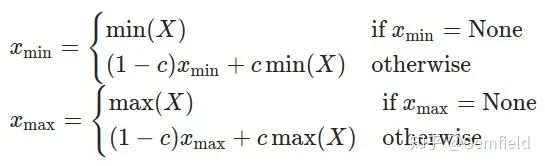
Xmin、Xmax是當(dāng)前運(yùn)行中正在求解和最終求解的最小值、最大值；
X是當(dāng)前輸入的tensor；
c是一個(gè)常數(shù)，PyTorch中默認(rèn)為0.01，也就是最新一次的極值由上一次貢獻(xiàn)99%，當(dāng)前的tensor貢獻(xiàn)1%。

MovingAverageMinMaxObserver在求min、max的方式和其基類MinMaxObserver有所區(qū)別之外，scale和zero_points的計(jì)算則是一致的。那么在包含了上述的observer之后，F(xiàn)akeQuantize的作用又是什么呢？看下面的步驟。

2，fuse_modules

和靜態(tài)量化一樣，不再贅述。

3，prepare_qat

在靜態(tài)量化中，我們這一步使用的是prepare API，而在QAT這里使用的是prepare_qat API。最重要的區(qū)別有兩點(diǎn)：

prepare_qat要把qconfig安插到每個(gè)op上，qconfig的內(nèi)容本身就不同，參考五部曲中的第一步；
prepare_qat 中需要多做一步轉(zhuǎn)換子module的工作，需要inplace的把模型中的一些子module替換了，替換的邏輯就是從DEFAULT_QAT_MODULE_MAPPINGS的key替換為value，這個(gè)字典的定義如下：

# Default map for swapping float module to qat modulesDEFAULT_QAT_MODULE_MAPPINGS : Dict[Callable, Any] = {    nn.Conv2d: nnqat.Conv2d,    nn.Linear: nnqat.Linear,    # Intrinsic modules:    nni.ConvBn1d: nniqat.ConvBn1d,    nni.ConvBn2d: nniqat.ConvBn2d,    nni.ConvBnReLU1d: nniqat.ConvBnReLU1d,    nni.ConvBnReLU2d: nniqat.ConvBnReLU2d,    nni.ConvReLU2d: nniqat.ConvReLU2d,    nni.LinearReLU: nniqat.LinearReLU}

因此，同靜態(tài)量化的prepare相比，prepare_qat在多插入fake_quants、又替換了nn.Conv2d、nn.Linear之后，CivilNet網(wǎng)絡(luò)就被改成了如下的樣子：

CivilNet(  (conv): QATConv2d(    1, 1, kernel_size=(1, 1), stride=(1, 1), bias=False    (activation_post_process): FakeQuantize(      fake_quant_enabled=tensor([1], dtype=torch.uint8), observer_enabled=tensor([1], dtype=torch.uint8),            scale=tensor([1.]), zero_point=tensor([0])      (activation_post_process): MovingAverageMinMaxObserver(min_val=tensor([]), max_val=tensor([]))    )    (weight_fake_quant): FakeQuantize(      fake_quant_enabled=tensor([1], dtype=torch.uint8), observer_enabled=tensor([1], dtype=torch.uint8),            scale=tensor([1.]), zero_point=tensor([0])      (activation_post_process): MovingAveragePerChannelMinMaxObserver(min_val=tensor([]), max_val=tensor([]))    )  )  (fc): QATLinear(    in_features=3, out_features=2, bias=False    (activation_post_process): FakeQuantize(      fake_quant_enabled=tensor([1], dtype=torch.uint8), observer_enabled=tensor([1], dtype=torch.uint8),            scale=tensor([1.]), zero_point=tensor([0])      (activation_post_process): MovingAverageMinMaxObserver(min_val=tensor([]), max_val=tensor([]))    )    (weight_fake_quant): FakeQuantize(      fake_quant_enabled=tensor([1], dtype=torch.uint8), observer_enabled=tensor([1], dtype=torch.uint8),            scale=tensor([1.]), zero_point=tensor([0])      (activation_post_process): MovingAveragePerChannelMinMaxObserver(min_val=tensor([]), max_val=tensor([]))    )  )  (relu): ReLU(    (activation_post_process): FakeQuantize(      fake_quant_enabled=tensor([1], dtype=torch.uint8), observer_enabled=tensor([1], dtype=torch.uint8),            scale=tensor([1.]), zero_point=tensor([0])      (activation_post_process): MovingAverageMinMaxObserver(min_val=tensor([]), max_val=tensor([]))    )  )  (quant): QuantStub(    (activation_post_process): FakeQuantize(      fake_quant_enabled=tensor([1], dtype=torch.uint8), observer_enabled=tensor([1], dtype=torch.uint8),            scale=tensor([1.]), zero_point=tensor([0])      (activation_post_process): MovingAverageMinMaxObserver(min_val=tensor([]), max_val=tensor([]))    )  )  (dequant): DeQuantStub())

4，喂數(shù)據(jù)

和靜態(tài)量化完全不同，在QAT中這一步是用來訓(xùn)練的。我們知道，在PyTorch的網(wǎng)絡(luò)中，前向推理邏輯都是實(shí)現(xiàn)在了每個(gè)op的forward函數(shù)中（參考：Gemfield：詳解Pytorch中的網(wǎng)絡(luò)構(gòu)造）（https://zhuanlan.zhihu.com/p/53927068）。而在prepare_qat中，所有的op被替換成了QAT版本的op，那么這些op的forward函數(shù)有什么特別的地方呢？

Conv2d被替換為了QATConv2d：

def forward(self, input):   return self.activation_post_process(self._conv_forward(input, self.weight_fake_quant(self.weight)))

Linear被替換為了QATLinear:

def forward(self, input):    return self.activation_post_process(F.linear(input, self.weight_fake_quant(self.weight), self.bias))

ReLU還是那個(gè)ReLU，不說了。總之，你可以看出來，每個(gè)op的輸入都需要經(jīng)過self.weight_fake_quant來處理下，輸出又都需要經(jīng)過self.activation_post_process來處理下，這兩個(gè)都是FakeQuantize的實(shí)例，只是里面包含的observer不一樣。以Conv2d為例：

#conv2dweight=functools.partial(<class 'torch.quantization.fake_quantize.FakeQuantize'>,            observer=<class 'torch.quantization.observer.MovingAveragePerChannelMinMaxObserver'>,            quant_min=-128, quant_max=127, dtype=torch.qint8,            qscheme=torch.per_channel_symmetric, reduce_range=False, ch_axis=0))
activation=functools.partial(<class 'torch.quantization.fake_quantize.FakeQuantize'>,             observer=<class 'torch.quantization.observer.MovingAverageMinMaxObserver'>,             quant_min=0, quant_max=255, reduce_range=True)

而FakeQuantize的forward函數(shù)如下所示：

def forward(self, X):        if self.observer_enabled[0] == 1:            #使用移動(dòng)平均算法計(jì)算scale和zp
        if self.fake_quant_enabled[0] == 1:            X = torch.fake_quantize_per_channel_or_tensor_affine(X...)        return X

FakeQuantize中的fake_quantize_per_channel_or_tensor_affine實(shí)現(xiàn)了quantize和dequantize，用公式表示的話為：out = (clamp(round(x/scale + zero_point), quant_min, quant_max)-zero_point)*scale。也就是說，這是把量化的誤差引入到了訓(xùn)練loss之中呀！

這樣，在QAT中，所有的weights和activations就像上面那樣被fake quantized了，且參與模型訓(xùn)練中的前向和反向計(jì)算。float值被round成了（用來模擬的）int8值，但是所有的計(jì)算仍然是通過float來完成的。這樣以來，所有的權(quán)重在優(yōu)化過程中都能感知到量化帶來的影響，稱之為量化感知訓(xùn)練（支持cpu和cuda），精度也因此更高。

5，轉(zhuǎn)換

這一步和靜態(tài)量化一樣，不再贅述。需要注意的是，QAT中，有一些module在prepare中已經(jīng)轉(zhuǎn)換成新的module了，所以靜態(tài)量化中所使用的字典包含有如下的條目：

DEFAULT_STATIC_QUANT_MODULE_MAPPINGS = {    ......    # QAT modules:    nnqat.Linear: nnq.Linear,    nnqat.Conv2d: nnq.Conv2d,}

總結(jié)下來就是：

# 原始的模型，所有的tensor和計(jì)算都是浮點(diǎn)previous_layer_fp32 -- linear_fp32 -- activation_fp32 -- next_layer_fp32                      /    linear_weight_fp32
# 訓(xùn)練過程中，fake_quants發(fā)揮作用previous_layer_fp32 -- fq -- linear_fp32 -- activation_fp32 -- fq -- next_layer_fp32                           /   linear_weight_fp32 -- fq
# 量化后的模型進(jìn)行推理，權(quán)重和輸入都是int8previous_layer_int8 -- linear_with_activation_int8 -- next_layer_int8                     /   linear_weight_int8

總結(jié)

那么如何更方便的在你的代碼中使用PyTorch的量化功能呢？一個(gè)比較優(yōu)雅的方式就是使用deepvac規(guī)范——這是一個(gè)定義了PyTorch工程標(biāo)準(zhǔn)的項(xiàng)目：

基于deepvac規(guī)范（包含庫），我們只需要簡單的打開幾個(gè)開關(guān)就可以使用上述的三種量化功能。

推薦閱讀

PyTorch模型量化工具學(xué)習(xí)
消除訓(xùn)練瓶頸，8點(diǎn)PyTorch提速技巧匯總
PyTorch 多機(jī)多卡訓(xùn)練：DDP 實(shí)戰(zhàn)與技巧

添加極市小助手微信（ID : cvmart2），備注：姓名-學(xué)校/公司-研究方向-城市（如：小極-北大-目標(biāo)檢測-深圳），即可申請加入極市目標(biāo)檢測/圖像分割/工業(yè)檢測/人臉/醫(yī)學(xué)影像/3D/SLAM/自動(dòng)駕駛/超分辨率/姿態(tài)估計(jì)/ReID/GAN/圖像增強(qiáng)/OCR/視頻理解等技術(shù)交流群：每月大咖直播分享、真實(shí)項(xiàng)目需求對接、求職內(nèi)推、算法競賽、干貨資訊匯總、與?10000+來自港科大、北大、清華、中科院、CMU、騰訊、百度等名校名企視覺開發(fā)者互動(dòng)交流~

△長按添加極市小助手

△長按關(guān)注極市平臺(tái)，獲取最新CV干貨

覺得有用麻煩給個(gè)在看啦~??

綜述：PyTorch的量化

背景

Tensor的量化

Post Training Dynamic Quantization

Post Training Static Quantization

QAT（Quantization Aware Training

總結(jié)