
讓你的單細(xì)胞數(shù)據(jù)動起來!|iCellR(二)
前情回顧:讓你的單細(xì)胞數(shù)據(jù)動起來!|iCellR(一)
在上文我們已經(jīng)基本完成了聚類分析和細(xì)胞在不同條件下的比例分析,下面繼續(xù)開始啦,讓你看看iCellR的強大!
1. 每個cluster的平均表達(dá)量
my.obj <- clust.avg.exp(my.obj)

head([email protected])
#      gene   cluster_1   cluster_2  cluster_3 cluster_4   cluster_5   cluster_6
#1     A1BG 0.072214723 0.092648973 0.08258609         0 0.027183115 0.072291636
#2 A1BG.AS1 0.014380756 0.003280237 0.01817982         0 0.000000000 0.011545546
#3     A1CF 0.000000000 0.000000000 0.00000000         0 0.000000000 0.000000000
#4      A2M 0.000000000 0.000000000 0.00000000         0 0.007004131 0.004672857
#5  A2M.AS1 0.003520828 0.039985296 0.00876364         0 0.056596203 0.018445562
#6    A2ML1 0.000000000 0.000000000 0.00000000         0 0.000000000 0.000000000
#   cluster_7  cluster_8   cluster_9
#1 0.09058946 0.04466827 0.027927923
#2 0.00000000 0.01534541 0.005930566
#3 0.00000000 0.00000000 0.000000000
#4 0.00000000 0.00000000 0.003411938
#5 0.00000000 0.00000000 0.000000000
#6 0.00000000 0.00000000 0.000000000
保存object
save(my.obj, file = "my.obj.Robj")2. 尋找marker基因
marker.genes <- findMarkers(my.obj,
    fold.change = 2,
    padjval = 0.1)   # 篩選條件

dim(marker.genes)
# [1] 1070   17

head(marker.genes)
#                row   baseMean    baseSD AvExpInCluster AvExpInOtherClusters
#LRRN3         LRRN3 0.01428477 0.1282046     0.05537243          0.003437002
#LINC00176 LINC00176 0.06757573 0.2949763     0.21404151          0.028906516
#FHIT           FHIT 0.10195359 0.3885343     0.31404936          0.045957058
#TSHZ2         TSHZ2 0.04831334 0.2628778     0.14300998          0.023311970
#CCR7           CCR7 0.28132627 0.6847417     0.81386444          0.140728033
#SCGB3A1     SCGB3A1 0.06319598 0.3554273     0.18130557          0.032013232
#          foldChange log2FoldChange         pval         padj clusters
#LRRN3      16.110677       4.009945 1.707232e-06 2.847662e-03        1
#LINC00176   7.404611       2.888424 4.189197e-16 7.117446e-13        1
#FHIT        6.833539       2.772633 1.576339e-19 2.681353e-16        1
#TSHZ2       6.134616       2.616973 8.613622e-10 1.455702e-06        1
#CCR7        5.783243       2.531879 1.994533e-42 3.400679e-39        1
#SCGB3A1     5.663457       2.501683 2.578484e-07 4.313805e-04        1
#               gene  cluster_1   cluster_2   cluster_3 cluster_4   cluster_5
#LRRN3         LRRN3 0.05537243 0.004102916 0.002190847         0 0.010902326
#LINC00176 LINC00176 0.21404151 0.016772401 0.005203161         0 0.009293024
#FHIT           FHIT 0.31404936 0.008713243 0.022934924         0 0.035701186
#TSHZ2         TSHZ2 0.14300998 0.008996236 0.009444180         0 0.000000000
#CCR7           CCR7 0.81386444 0.075719109 0.034017494         0 0.021492756
#SCGB3A1     SCGB3A1 0.18130557 0.039644151 0.001183264         0 0.000000000
#            cluster_6  cluster_7   cluster_8   cluster_9
#LRRN3     0.002087831 0.00000000 0.000000000 0.012113258
#LINC00176 0.086762509 0.01198777 0.003501552 0.003560614
#FHIT      0.104189143 0.04144293 0.041064681 0.007218861
#TSHZ2     0.065509372 0.01690584 0.002352707 0.015350123
#CCR7      0.272580821 0.06523324 0.257130255 0.031304151
#SCGB3A1   0.078878071 0.01198777 0.000000000 0.043410608

# baseMean: average expression in all the cells 所有細(xì)胞的平均表達(dá)值
# baseSD: Standard Deviation 標(biāo)準(zhǔn)偏差
# AvExpInCluster: average expression in cluster number (see clusters) 該cluster中的平均表達(dá)值
# AvExpInOtherClusters: average expression in all the other clusters  在所有其他cluster的平均表達(dá)值
# foldChange: AvExpInCluster/AvExpInOtherClusters  表達(dá)差異倍數(shù)
# log2FoldChange: log2(AvExpInCluster/AvExpInOtherClusters) 取表達(dá)差異倍數(shù)的log2的值
# pval: P value
# padj: Adjusted P value
# clusters: marker for cluster number
# gene: marker gene for the cluster cluster的marker gene
# the rest are the average expression for each cluster3. 繪制基因表達(dá)情況
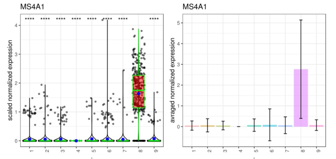
基因MS4A1:tSNE 2D,PCA 2D展示該基因在兩種降維方式下,每個組的平均表達(dá)分布圖。Box Plot和Bar plot展示了該基因在每個簇中的表達(dá)箱線圖和條形圖
# tSNE 2D
A <- gene.plot(my.obj, gene = "MS4A1",
    plot.type = "scatterplot",
    interactive = F,
    out.name = "scatter_plot")
# PCA 2D
B <- gene.plot(my.obj, gene = "MS4A1",
    plot.type = "scatterplot",
    interactive = F,
    out.name = "scatter_plot",
    plot.data.type = "pca")

# Box Plot
C <- gene.plot(my.obj, gene = "MS4A1",
    box.to.test = 0,
    box.pval = "sig.signs",
    col.by = "clusters",
    plot.type = "boxplot",
    interactive = F,
    out.name = "box_plot")

# Bar plot (to visualize fold changes)
D <- gene.plot(my.obj, gene = "MS4A1",
    col.by = "clusters",
    plot.type = "barplot",
    interactive = F,
    out.name = "bar_plot")

library(gridExtra)
grid.arrange(A,B,C,D) # 4個圖合并展示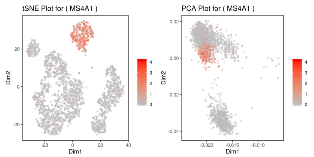
展示多個基因的plots:
genelist = c("PPBP","LYZ","MS4A1","GNLY","LTB","NKG7","IFITM2","CD14","S100A9")
###
for(i in genelist){
    MyPlot <- gene.plot(my.obj, gene = i,
        interactive = F,
        plot.data.type = "umap",
        cell.transparency = 1)
    NameCol=paste("PL",i,sep="_")
    eval(call("<-", as.name(NameCol), MyPlot))
}
###
library(cowplot)
filenames <- ls(pattern="PL_")
plot_grid(plotlist=mget(filenames[1:9]))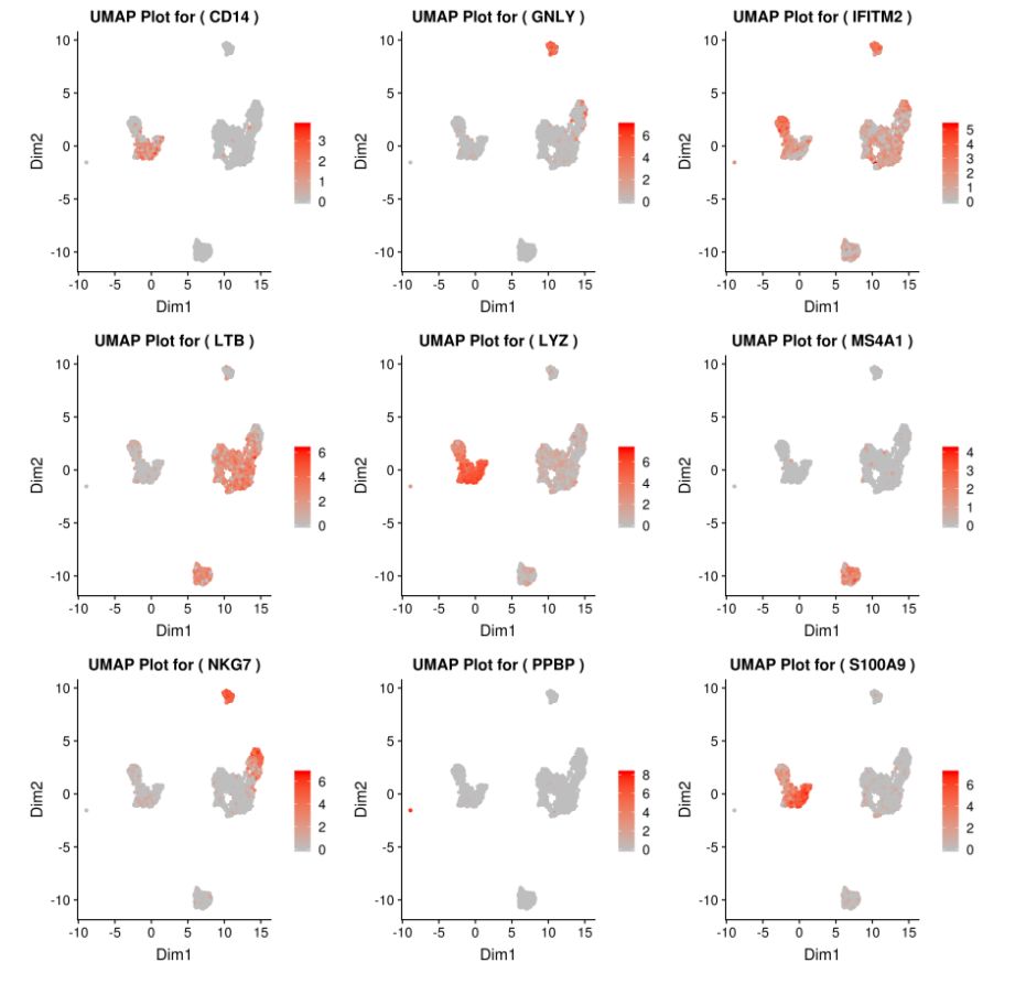
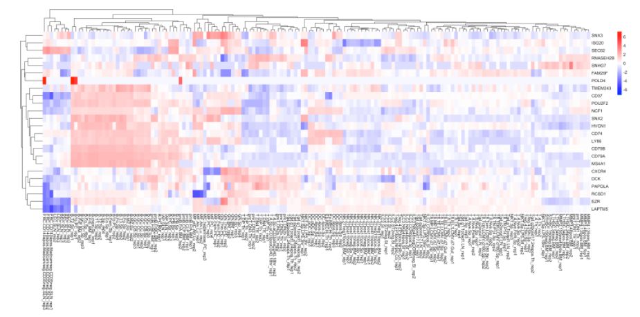
熱圖分析:
# 獲取top10高變基因
MyGenes <- top.markers(marker.genes, topde = 10, min.base.mean = 0.2,filt.ambig = F)
MyGenes <- unique(MyGenes)
# plot
heatmap.gg.plot(my.obj, gene = MyGenes, interactive = T, out.name = "plot", cluster.by = "clusters")
# or
heatmap.gg.plot(my.obj, gene = MyGenes, interactive = F, cluster.by = "clusters")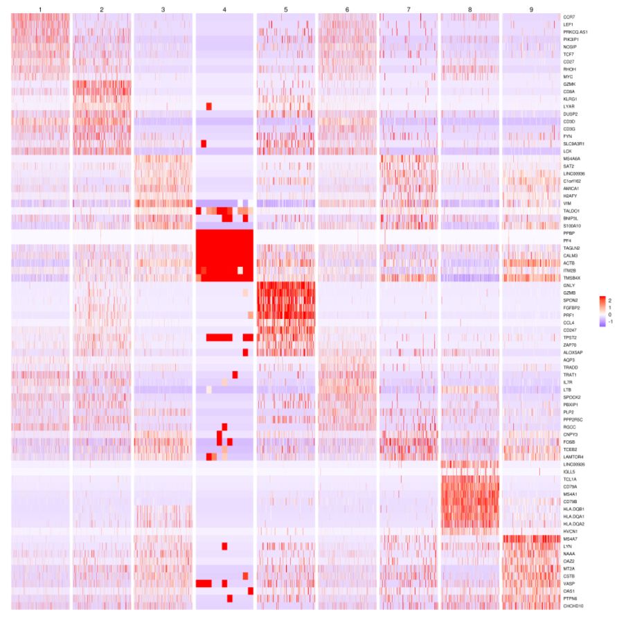
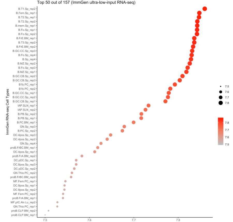
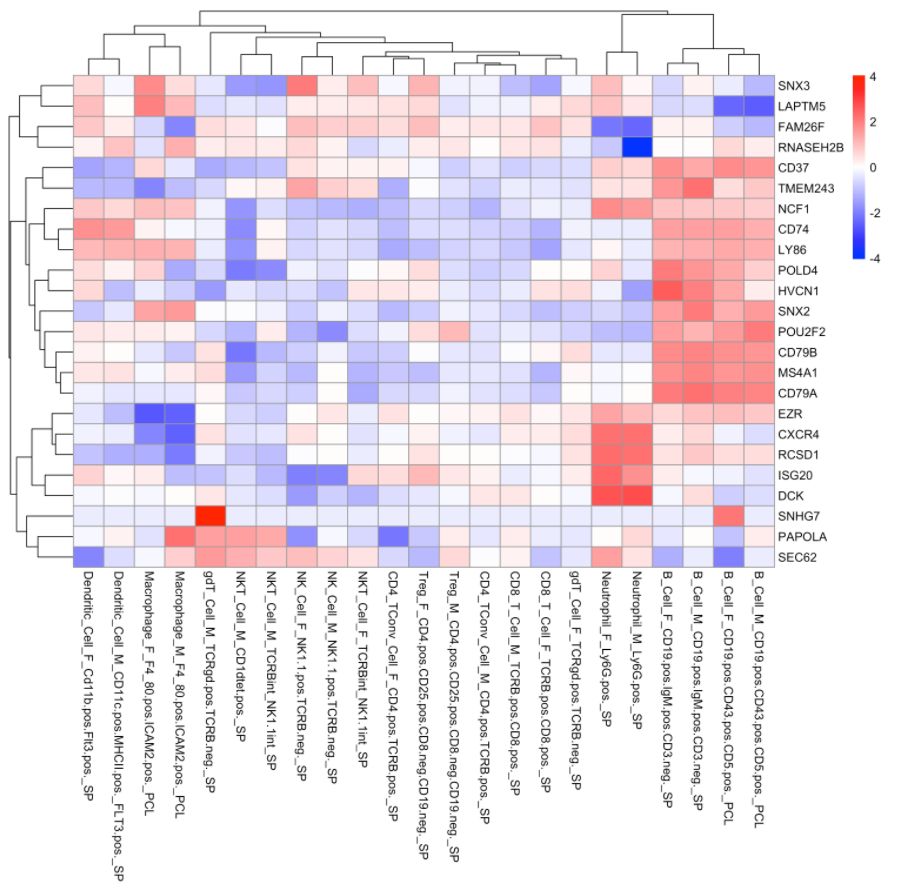
4. 使用ImmGen進(jìn)行細(xì)胞類型預(yù)測
注意:ImmGen是小鼠基因組數(shù)據(jù),此處的樣本數(shù)據(jù)是人的。對于157個ULI-RNA-Seq(Ultra-low-input RNA-seq)樣本,使用的metadata是:
https://github.com/rezakj/scSeqR/blob/dev/doc/uli_RNA_metadat.txt
# 繪制cluster8中top40基因(平均表達(dá)值最小為0.2)在不同細(xì)胞的表達(dá)分布圖
Cluster = 8
MyGenes <- top.markers(marker.genes, topde = 40, min.base.mean = 0.2, cluster = Cluster)
# 畫圖
cell.type.pred(immgen.data = "rna", gene = MyGenes, plot.type = "point.plot")
# and
cell.type.pred(immgen.data = "uli.rna", gene = MyGenes, plot.type = "point.plot", top.cell.types = 50)
# or
cell.type.pred(immgen.data = "rna", gene = MyGenes, plot.type = "heatmap")
# and
cell.type.pred(immgen.data = "uli.rna", gene = MyGenes, plot.type = "heatmap")

# And finally check the genes in the cells and find the common ones to predict
# heatmap.gg.plot(my.obj, gene = MyGenes, interactive = F, cluster.by = "clusters")

# 可以看出來cluster 8更像B細(xì)胞!# for tissue type prediction use this:
#cell.type.pred(immgen.data = "mca", gene = MyGenes, plot.type = "point.plot")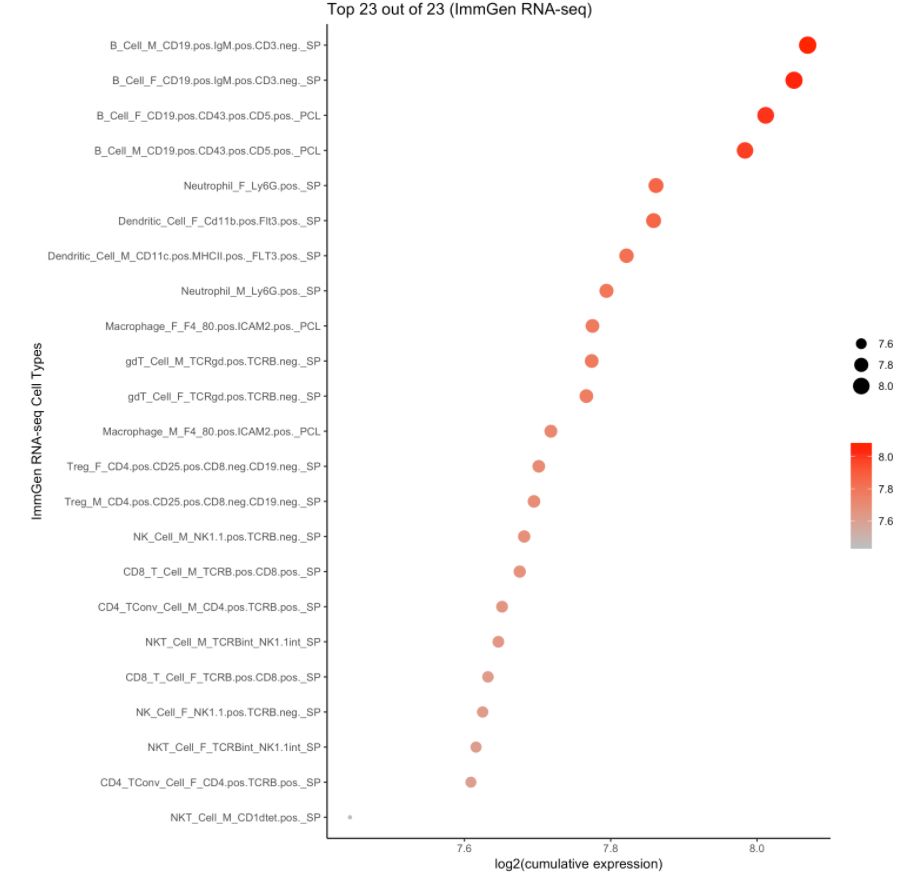
5. Pathway analysis
# cluster7的KEGG Pathway
# pathways.kegg(my.obj, clust.num = 7)
# this function is being improved and soon will be available 這個函數(shù)還要改進(jìn),很快就能用了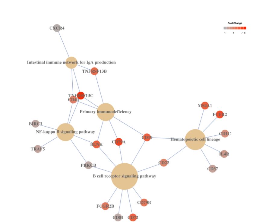
對cluster進(jìn)行QC:
clust.stats.plot(my.obj, plot.type = "box.mito", interactive = F)  # 每個cluster中細(xì)胞的線粒體基因分布圖
clust.stats.plot(my.obj, plot.type = "box.gene", interactive = F)  # 每個cluster中細(xì)胞的基因分布圖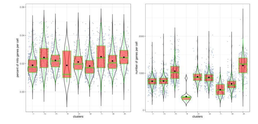
6. 差異表達(dá)分析
diff.res <- run.diff.exp(my.obj, de.by = "clusters", cond.1 = c(1,4), cond.2 = c(2))  # cluster之間的比較得到差異表達(dá)基因
diff.res1 <- as.data.frame(diff.res)
diff.res1 <- subset(diff.res1, padj < 0.05)   # 篩選padj < 0.05的基因
head(diff.res1)
#             baseMean        1_4           2 foldChange log2FoldChange         pval
#AAK1       0.19554589 0.26338228 0.041792762 0.15867719      -2.655833 8.497012e-33
#ABHD14A    0.09645732 0.12708519 0.027038379 0.21275791      -2.232715 1.151865e-11
#ABHD14B    0.19132829 0.23177944 0.099644572 0.42991118      -1.217889 3.163623e-09
#ABLIM1     0.06901900 0.08749258 0.027148089 0.31029018      -1.688310 1.076382e-06
#AC013264.2 0.07383608 0.10584821 0.001279649 0.01208947      -6.370105 1.291674e-19
#AC092580.4 0.03730859 0.05112053 0.006003441 0.11743700      -3.090041 5.048838e-07
                   padj
#AAK1       1.294690e-28
#ABHD14A    1.708446e-07
#ABHD14B    4.636290e-05
#ABLIM1     1.540087e-02
#AC013264.2 1.950557e-15
#AC092580.4 7.254675e-03

# more examples 注意參數(shù)“de.by”設(shè)置的是不同差異比較方式
diff.res <- run.diff.exp(my.obj, de.by = "conditions", cond.1 = c("WT"), cond.2 = c("KO"))  #  WT vs KO
diff.res <- run.diff.exp(my.obj, de.by = "clusters", cond.1 = c(1,4), cond.2 = c(2))  # cluster 1 and 2 vs. 4
diff.res <- run.diff.exp(my.obj, de.by = "clustBase.condComp", cond.1 = c("WT"), cond.2 = c("KO"), base.cond = 1)  #  cluster 1 WT vs cluster 1 KO
diff.res <- run.diff.exp(my.obj, de.by = "condBase.clustComp", cond.1 = c(1), cond.2 = c(2), base.cond = "WT") # cluster 1 vs cluster 2 but only the WT sample
畫差異表達(dá)基因的火山圖和MA圖:
# Volcano Plot
volcano.ma.plot(diff.res,
    sig.value = "pval",
    sig.line = 0.05,
    plot.type = "volcano",
    interactive = F)

# MA Plot
volcano.ma.plot(diff.res,
    sig.value = "pval",
    sig.line = 0.05,
    plot.type = "ma",
    interactive = F)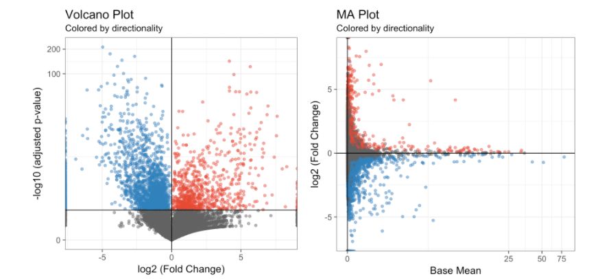
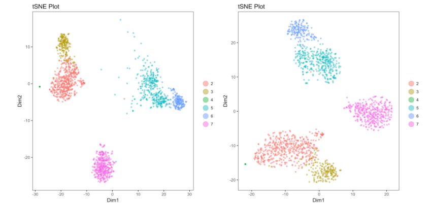
7. 合并,重置,重命名和刪除cluster
# 如果你想要合并cluster 2和cluster 3
my.obj <- change.clust(my.obj, change.clust = 3, to.clust = 2)

# 重置為原來的分類
my.obj <- change.clust(my.obj, clust.reset = T)

# 可以將cluster7編號重命名為細(xì)胞類型-"B Cell".
my.obj <- change.clust(my.obj, change.clust = 7, to.clust = "B Cell")

# 刪除cluster1
my.obj <- clust.rm(my.obj, clust.to.rm = 1)

# 進(jìn)行tSNE對細(xì)胞重新定位
my.obj <- run.tsne(my.obj, clust.method = "gene.model", gene.list = "my_model_genes.txt")

# Use this for plotting as you make the changes
cluster.plot(my.obj,
   cell.size = 1,
   plot.type = "tsne",
   cell.color = "black",
   back.col = "white",
   col.by = "clusters",
   cell.transparency = 0.5,
   clust.dim = 2,
   interactive = F)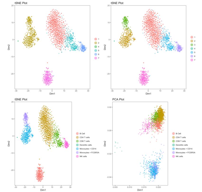
Cell gating:可以框出指定的信息
my.plot <- gene.plot(my.obj, gene = "GNLY",
  plot.type = "scatterplot",
  clust.dim = 2,
  interactive = F)

cell.gating(my.obj, my.plot = my.plot)

# or

#my.plot <- cluster.plot(my.obj,
#    cell.size = 1,
#    cell.transparency = 0.5,
#    clust.dim = 2,
#    interactive = F)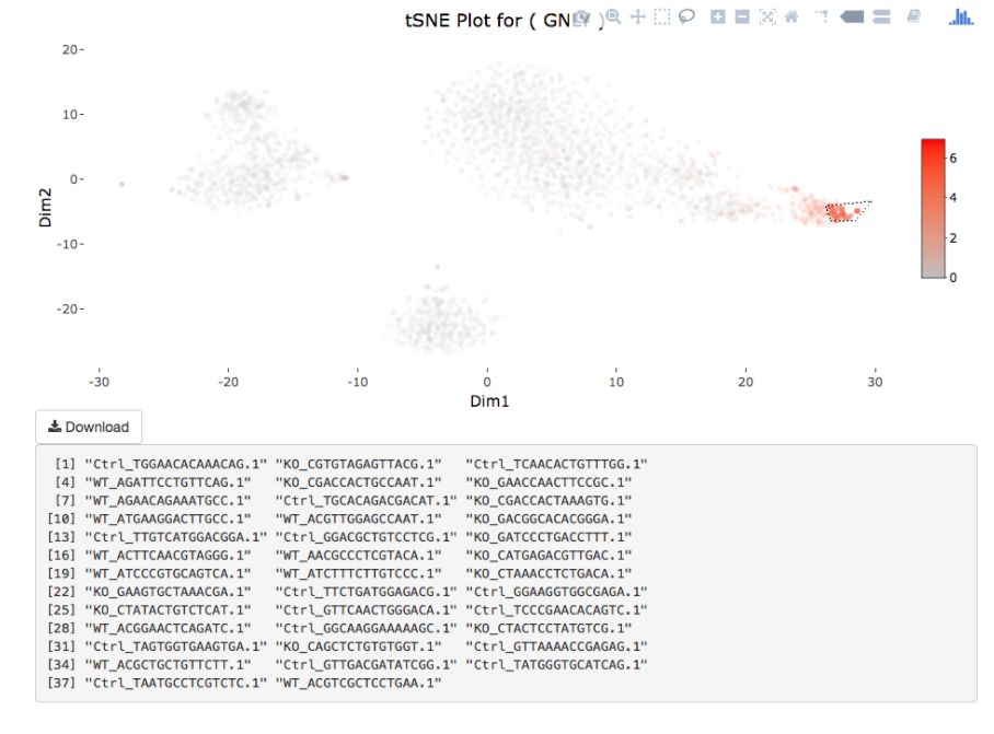
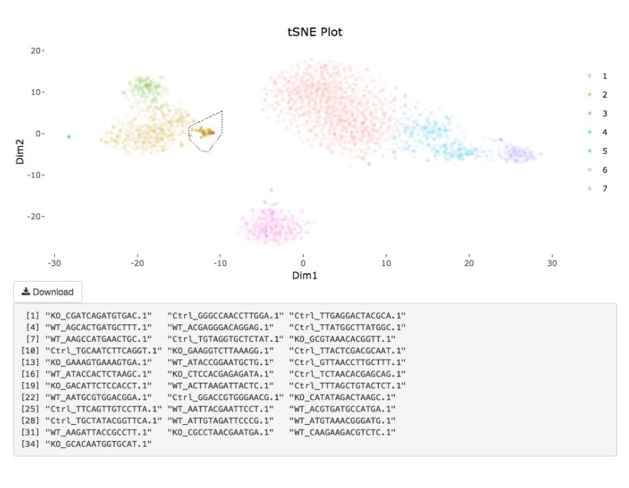
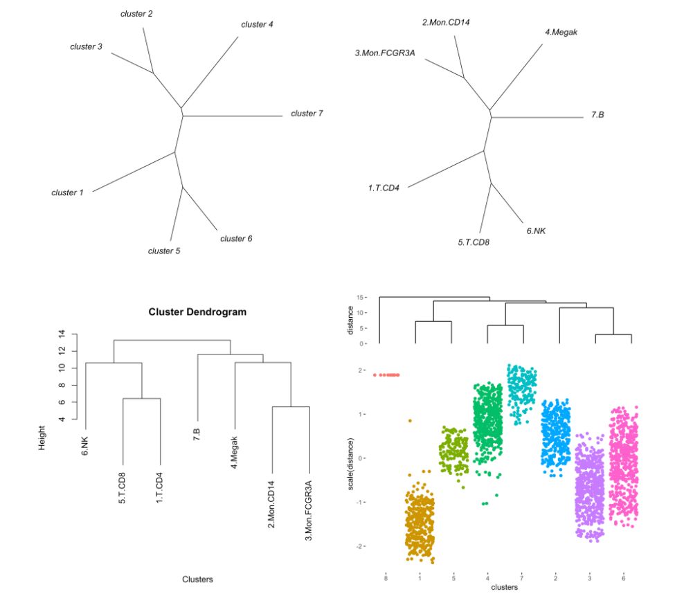
my.obj <- gate.to.clust(my.obj, my.gate = "cellGating.txt", to.clust = 10)8. 偽時序分析
注意參數(shù)“type”
MyGenes <- top.markers(marker.genes, topde = 50, min.base.mean = 0.2)
MyGenes <- unique(MyGenes)

pseudotime.tree(my.obj,
   marker.genes = MyGenes,
   type = "unrooted",
   clust.method = "complete")

# or

pseudotime.tree(my.obj,
   marker.genes = MyGenes,
   type = "classic",
   clust.method = "complete")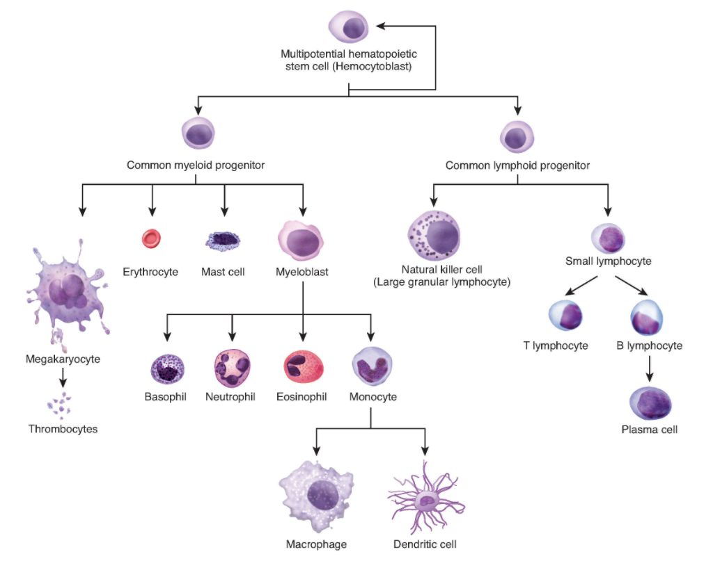
9. 應(yīng)用monocle進(jìn)行偽時序分析
library(monocle)

MyMTX <- [email protected]
GeneAnno <- as.data.frame(row.names(MyMTX))
colnames(GeneAnno) <- "gene_short_name"
row.names(GeneAnno) <- GeneAnno$gene_short_name
cell.cluster <- ([email protected])
Ha <- data.frame(do.call('rbind', strsplit(as.character(row.names(cell.cluster)),'_',fixed=TRUE)))[1]
clusts <- paste("cl.",as.character(cell.cluster$clusters),sep="")
cell.cluster <- cbind(cell.cluster,Ha,clusts)
colnames(cell.cluster) <- c("Clusts","iCellR.Conds","iCellR.Clusts")
Samp <- new("AnnotatedDataFrame", data = cell.cluster)
Anno <- new("AnnotatedDataFrame", data = GeneAnno)
my.monoc.obj <- newCellDataSet(as.matrix(MyMTX),phenoData = Samp, featureData = Anno)

## find disperesedgenes
my.monoc.obj <- estimateSizeFactors(my.monoc.obj)
my.monoc.obj <- estimateDispersions(my.monoc.obj)
disp_table <- dispersionTable(my.monoc.obj)

unsup_clustering_genes <- subset(disp_table, mean_expression >= 0.1)
my.monoc.obj <- setOrderingFilter(my.monoc.obj, unsup_clustering_genes$gene_id)

# tSNE
my.monoc.obj <- reduceDimension(my.monoc.obj, max_components = 2, num_dim = 10,reduction_method = 'tSNE', verbose = T)
# cluster
my.monoc.obj <- clusterCells(my.monoc.obj, num_clusters = 10)

## plot conditions and clusters based on iCellR analysis
A <- plot_cell_clusters(my.monoc.obj, 1, 2, color = "iCellR.Conds")
B <- plot_cell_clusters(my.monoc.obj, 1, 2, color = "iCellR.Clusts")

## plot clusters based monocle analysis
C <- plot_cell_clusters(my.monoc.obj, 1, 2, color = "Cluster")

# get marker genes from iCellR analysis
MyGenes <- top.markers(marker.genes, topde = 30, min.base.mean = 0.2)
my.monoc.obj <- setOrderingFilter(my.monoc.obj, MyGenes)

my.monoc.obj <- reduceDimension(my.monoc.obj, max_components = 2,method = 'DDRTree')
# order cells
my.monoc.obj <- orderCells(my.monoc.obj)

# plot based on iCellR analysis and marker genes from iCellR
D <- plot_cell_trajectory(my.monoc.obj, color_by = "iCellR.Clusts")

## heatmap genes from iCellR

plot_pseudotime_heatmap(my.monoc.obj[MyGenes,],
  cores = 1,
  cluster_rows = F,
  use_gene_short_name = T,
  show_rownames = T)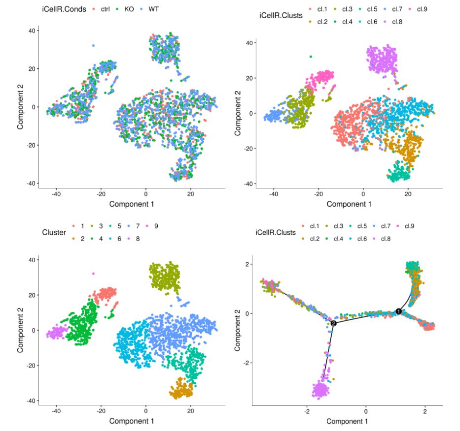
10. iCellR應(yīng)用于scVDJ-seq數(shù)據(jù)
# first prepare the files.
# this function would filter the files, calculate clonotype frequencies and proportions and add conditions to the cell ids.
my.vdj.1 <- prep.vdj(vdj.data = "all_contig_annotations.csv", cond.name = "WT")
my.vdj.2 <- prep.vdj(vdj.data = "all_contig_annotations.csv", cond.name = "KO")
my.vdj.3 <- prep.vdj(vdj.data = "all_contig_annotations.csv", cond.name = "Ctrl")

# concatenate all the conditions
my.vdj.data <- rbind(my.vdj.1, my.vdj.2, my.vdj.3)

# see head of the file
head(my.vdj.data)
#  raw_clonotype_id               barcode is_cell                   contig_id
#1       clonotype1 WT_AAACCTGAGCTAACTC-1    True AAACCTGAGCTAACTC-1_contig_1
#2       clonotype1 WT_AAACCTGAGCTAACTC-1    True AAACCTGAGCTAACTC-1_contig_2
#3       clonotype1 WT_AGTTGGTTCTCGCATC-1    True AGTTGGTTCTCGCATC-1_contig_3
#4       clonotype1 WT_TGACAACCAACTGCTA-1    True TGACAACCAACTGCTA-1_contig_1
#5       clonotype1 WT_TGTCCCAGTCAAACTC-1    True TGTCCCAGTCAAACTC-1_contig_1
#6       clonotype1 WT_TGTCCCAGTCAAACTC-1    True TGTCCCAGTCAAACTC-1_contig_2
#  high_confidence length chain  v_gene d_gene  j_gene c_gene full_length
#1            True    693   TRA TRAV8-1   None  TRAJ21   TRAC        True
#2            True    744   TRB  TRBV28  TRBD1 TRBJ2-1  TRBC2        True
#3            True    647   TRA TRAV8-1   None  TRAJ21   TRAC        True
#4            True    508   TRB  TRBV28  TRBD1 TRBJ2-1  TRBC2        True
#5            True    660   TRA TRAV8-1   None  TRAJ21   TRAC        True
#6            True    770   TRB  TRBV28  TRBD1 TRBJ2-1  TRBC2        True
#  productive             cdr3                                          cdr3_nt
#1       True      CAVKDFNKFYF                TGTGCCGTGAAAGACTTCAACAAATTTTACTTT
#2       True CASSLFSGTGTNEQFF TGTGCCAGCAGTTTATTTTCCGGGACAGGGACGAATGAGCAGTTCTTC
#3       True      CAVKDFNKFYF                TGTGCCGTGAAAGACTTCAACAAATTTTACTTT
#4       True CASSLFSGTGTNEQFF TGTGCCAGCAGTTTATTTTCCGGGACAGGGACGAATGAGCAGTTCTTC
#5       True      CAVKDFNKFYF                TGTGCCGTGAAAGACTTCAACAAATTTTACTTT
#6       True CASSLFSGTGTNEQFF TGTGCCAGCAGTTTATTTTCCGGGACAGGGACGAATGAGCAGTTCTTC
#  reads umis       raw_consensus_id my.raw_clonotype_id clonotype.Freq
#1  1241    2 clonotype1_consensus_1          clonotype1            120
#2  2400    4 clonotype1_consensus_2          clonotype1            120
#3  1090    2 clonotype1_consensus_1          clonotype1            120
#4  2455    4 clonotype1_consensus_2          clonotype1            120
#5  1346    2 clonotype1_consensus_1          clonotype1            120
#6  3073    8 clonotype1_consensus_2          clonotype1            120
#  proportion total.colonotype
#1 0.04098361             1292
#2 0.04098361             1292
#3 0.04098361             1292
#4 0.04098361             1292
#5 0.04098361             1292
#6 0.04098361             1292

# add it to iCellR object
add.vdj(my.obj, vdj.data = my.vdj.data)
reference
如果想嘗試一下,這里有傳送門哦!
https://github.com/rezakj/iCellR
推薦閱讀
學(xué)習(xí)津貼
單篇留言點贊數(shù)的第一位(點贊數(shù)至少為8)可獲得我們贈送的在線基礎(chǔ)課的9折優(yōu)惠券。
越留言,越幸運。
主編會在每周選擇一位最有深度的留言,評論者可獲得我們贈送的任意一門在線課程的9折優(yōu)惠券(偷偷告訴你,這個任意是由你選擇哦)。
高顏值免費在線繪圖
往期精品
心得體會?TCGA數(shù)據(jù)庫?Linux?Python?
生信學(xué)習(xí)視頻?PPT?EXCEL?文章寫作?ggplot2
自學(xué)生信?2019影響因子?GSEA?單細(xì)胞?
后臺回復(fù)“生信寶典福利第一波”或點擊閱讀原文獲取教程合集