用python做時間序列預(yù)測十:時間序列實踐-航司乘客數(shù)預(yù)測

本文以航司乘客數(shù)預(yù)測的例子來組織相關(guān)時間序列預(yù)測的代碼，通過了解本文中的代碼，當遇到其它場景的時間序列預(yù)測亦可套用。

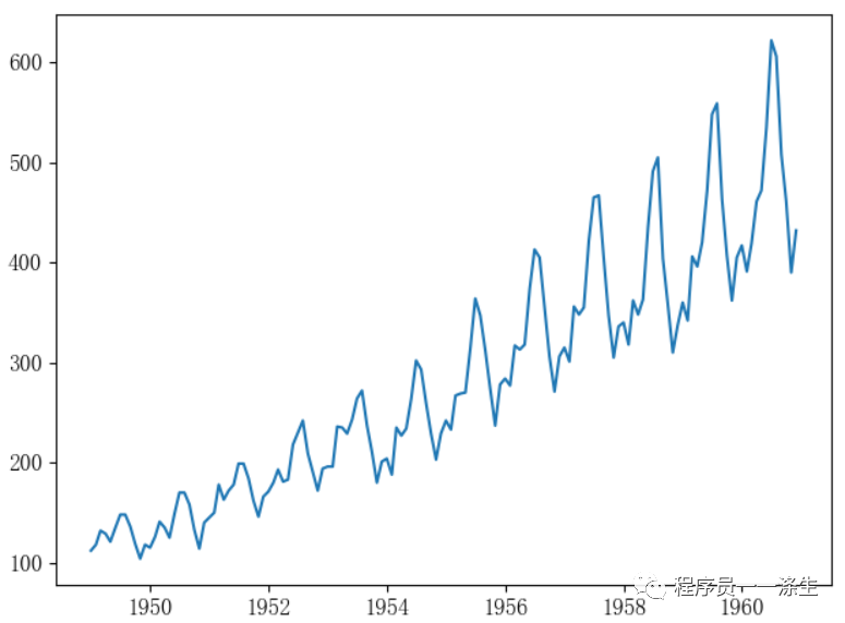
航司乘客數(shù)序列

預(yù)測步驟

# 加載時間序列數(shù)據(jù)
_ts = load_data()
# 使用樣本熵評估可預(yù)測性
print(f'原序列樣本熵:{SampEn(_ts.values, m=2, r=0.2 * np.std(_ts.values))}')
# 檢驗平穩(wěn)性
use_rolling_statistics(_ts)  # rolling 肉眼
use_df(_ts)  # Dickey-Fuller Test 量化
# 平穩(wěn)變換
_ts_log, _rs_log_diff = transform_stationary(_ts)
# 使用樣本熵評估可預(yù)測性
print(f'平穩(wěn)變換后的序列樣本熵:{SampEn(_ts.values, m=2, r=0.2 * np.std(_ts.values))}')
# acf,pacf定階分析
order_determination(_rs_log_diff)
# plot_lag(_rs)# lag plot(滯后圖分析相關(guān)性)
# 構(gòu)建模型
_fittedvalues, _fc, _conf, _title = build_arima(
    _ts_log)  # 這里只傳取log后的序列是因為后面會通過指定ARIMA模型的參數(shù)d=1來做一階差分，這樣在預(yù)測的時候，就不需要手動做逆差分來還原序列，而是由ARIMA模型自動還原
# 預(yù)測,并繪制預(yù)測結(jié)果圖
transform_back(_ts, _fittedvalues, _fc, _conf, _title)

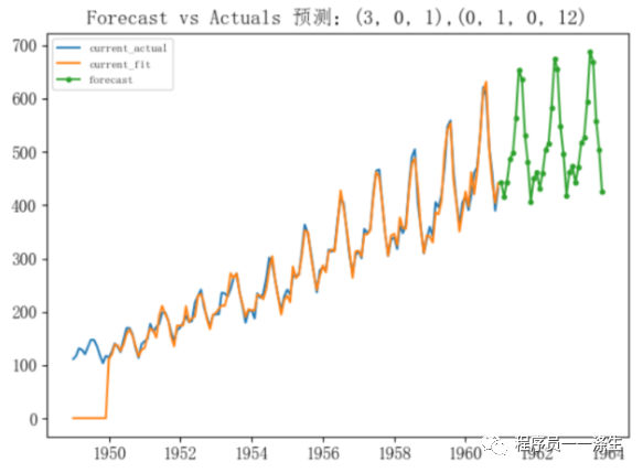
預(yù)測結(jié)果

完整代碼

# coding='utf-8'
"""
航司乘客數(shù)時間序列數(shù)據(jù)集
該數(shù)據(jù)集包含了1949-1960年每個月國際航班的乘客總數(shù)。
"""
import numpy as np
from matplotlib import rcParams
from statsmodels.tsa.seasonal import seasonal_decompose
from statsmodels.tsa.statespace.sarimax import SARIMAX
from statsmodels.tsa.stattools import acf, pacf

params = {'font.family': 'serif',
'font.serif': 'FangSong',
'font.style': 'italic',
'font.weight': 'normal',  # or 'blod'
'font.size': 12,  # 此處貌似不能用類似large、small、medium字符串
'axes.unicode_minus': False
          }
rcParams.update(params)
import matplotlib.pyplot as plt
import pandas as pd
# 未來pandas版本會要求顯式注冊matplotlib的轉(zhuǎn)換器，所以添加了下面兩行代碼，否則會報警告
from pandas.plotting import register_matplotlib_converters

register_matplotlib_converters()


def load_data():
from datetime import datetime
    date_parse = lambda x: datetime.strptime(x, '%Y-%m-%d')
    data = pd.read_csv('datas/samples/AirPassengers.csv',
                       index_col='Month',  # 指定索引列
                       parse_dates=['Month'],  # 將指定列按照日期格式來解析
                       date_parser=date_parse  # 日期格式解析器
                       )
    ts = data['y']
    print(ts.head(10))
    plt.plot(ts)
    plt.show()
return ts


def use_rolling_statistics(time_series_datas):
'''
    利用標準差和均值來肉眼觀測時間序列數(shù)據(jù)的平穩(wěn)情況
    :param time_series_datas:
    :return:
    '''
    roll_mean = time_series_datas.rolling(window=12).mean()
    roll_std = time_series_datas.rolling(window=12).std()
# roll_variance = time_series_datas.rolling(window=12).var()
    plt.plot(time_series_datas, color='blue', label='Original')
    plt.plot(roll_mean, color='red', label='Rolling Mean')
    plt.plot(roll_std, color='green', label='Rolling Std')
# plt.plot(roll_variance,color='yellow',label='Rolling Variance')

    plt.legend(loc='best')
    plt.title('利用Rolling Statistics來觀測時間序列數(shù)據(jù)的平穩(wěn)情況')
    plt.show(block=False)


def use_df(time_series_datas):
'''
    迪基-富勒單位根檢驗
    :param time_series_datas:
    :return:
    '''
from statsmodels.tsa.stattools import adfuller
    dftest = adfuller(time_series_datas, autolag='AIC')
    dfoutput = pd.Series(dftest[0:4], index=['Test Statistic', 'p-value', '#Lags Used', 'Number of Observations Used'])
for key, value in dftest[4].items():
        dfoutput['Critical Value (%s)' % key] = value
    print(dfoutput)


def use_moving_avg(ts_log):
    moving_avg_month = ts_log.rolling(window=12).mean()
    plt.plot(moving_avg_month, color='green', label='moving_avg')
    plt.legend(loc='best')
    plt.title('利用移動平均法平滑ts_log序列')
    plt.show()
return moving_avg_month


def use_exponentially_weighted_moving_avg(ts_log):
    expweighted_avg = ts_log.ewm(halflife=12).mean()
    plt.plot(expweighted_avg, color='green', label='expweighted_avg')
    plt.legend(loc='best')
    plt.title('利用指數(shù)加權(quán)移動平均法平滑ts_log序列')
    plt.show()
return expweighted_avg


def use_decomposition(ts_log):
'''
    時間序列分解
    :param ts_log:
    :return: 去除不平穩(wěn)因素后的序列
    '''
    decomposition = seasonal_decompose(ts_log, freq=12)
    trend = decomposition.trend
    seasonal = decomposition.seasonal
    residual = decomposition.resid

    plt.subplot(411)
    plt.plot(ts_log, label='Original')
    plt.legend(loc='best')
    plt.subplot(412)
    plt.plot(trend, label='Trend')
    plt.legend(loc='best')
    plt.subplot(413)
    plt.plot(seasonal, label='Seasonality')
    plt.legend(loc='best')
    plt.subplot(414)
    plt.plot(residual, label='Residuals')
    plt.legend(loc='best')
    plt.tight_layout()
    plt.show()
# 衡量趨勢強度
    r_var = residual.var()
    tr_var = (trend + residual).var()
    f_t = np.maximum(0, 1.0 - r_var / tr_var)
    print(f_t)
# 衡量季節(jié)性強度
    sr_var = (seasonal + residual).var()
    f_s = np.maximum(0, 1.0 - r_var / sr_var)
    print(f"-------趨勢強度:{f_t},季節(jié)性強度:{f_s}------")
return residual


def transform_stationary(ts):
'''
    平穩(wěn)變換：
    消除趨勢：移動平均、指數(shù)加權(quán)移動平均
    有時候簡單的減掉趨勢的方法并不能得到平穩(wěn)序列，尤其對于高季節(jié)性的時間序列來說，此時可以采用differencing(差分)或decomposition(分解)
    消除趨勢和季節(jié)性：差分、序列分解
    :param ts:
    :return:
    '''
# 利用log降低異方差性
    ts_log = np.log(ts)
# plt.plot(ts_log, color='brown', label='ts_log')
# plt.title('ts_log')
# plt.show()

# 移動平均法，得到趨勢（需要確定合適的K值，當前例子中，合適的K值是12個月，因為趨勢是逐年增長，但是有些復(fù)雜場景下，K值的確定很難）
# trend = use_moving_avg(ts_log)
# 指數(shù)加權(quán)移動平均法平，得到趨勢(由于每次都是從當前時刻到起始時刻的指數(shù)加權(quán)平均，所以沒有確定K值的問題)
# trend = use_exponentially_weighted_moving_avg(ts_log)
# print(trend)
# 減去趨勢：將平滑后的序列從ts_log序列中移除
# rs = ts_log - trend
# 若趨勢建模是用的移動平均法，由于是取前12個月的均值，所以開始的11個值的移動平均都是非數(shù)了，需要去除非數(shù)
# rs.dropna(inplace=True)

# differencing(差分)
    rs_log_diff = ts_log - ts_log.shift()  # 1階差分
# use_rolling_statistics(rs)
# rs = rs - rs.shift() # 2階差分
# 季節(jié)性差分 ,此案例中的季節(jié)間隔為12個月  d=1 D=1
# rs = (ts_log - ts_log.shift(periods=12)) - (ts_log.shift() - ts_log.shift().shift(periods=12))
    rs_log_diff.dropna(inplace=True)

# decomposition(分解)
# rs = use_decomposition(ts_log)
# rs.dropna(inplace=True)

# 對去除趨勢后的序列做平穩(wěn)性檢驗
# use_rolling_statistics(rs)
    use_df(rs_log_diff)
return ts_log, rs_log_diff


def order_determination(ts_log_diff):
'''
    利用acf和pacf確定模型以及階數(shù)
    :param ts_log_diff:
    :return:
    '''
    lag_acf = acf(ts_log_diff, nlags=10, fft=False)
    lag_pacf = pacf(ts_log_diff, nlags=10, method='ols')
    z = 1.96
# z = 1.65
# Plot ACF:
    plt.subplot(121)
    plt.plot(lag_acf)
    plt.axhline(y=0, linestyle='--', color='gray')
    plt.axhline(y=-z / np.sqrt(len(ts_log_diff) - 1), linestyle='--',
                color='gray')  # 利用白噪聲的標準正態(tài)分布假設(shè)來選擇相關(guān)性的置信度區(qū)間，1.96是95%置信度下的統(tǒng)計量
    plt.axhline(y=z / np.sqrt(len(ts_log_diff) - 1), linestyle='--', color='gray')
    plt.title('Autocorrelation Function')
# Plot PACF:
    plt.subplot(122)
    plt.plot(lag_pacf)
    plt.axhline(y=0, linestyle='--', color='gray')
    plt.axhline(y=-z / np.sqrt(len(ts_log_diff)), linestyle='--', color='gray')
    plt.axhline(y=z / np.sqrt(len(ts_log_diff)), linestyle='--', color='gray')
    plt.title('Partial Autocorrelation Function')
    plt.tight_layout()
    plt.show()


def draw_rss_plot(ts_log_diff, orders, title, freq='MS'):
from statsmodels.tsa.arima_model import ARIMA
    model = ARIMA(ts_log_diff, order=orders, freq=freq)
    results_fitted = model.fit(disp=-1)
# print(results.summary())
    plt.plot(ts_log_diff)
    plt.plot(results_fitted.fittedvalues, color='red')
    plt.title('%s RSS: %.4f' % (title, sum((results_fitted.fittedvalues - ts_log_diff) ** 2)))
    plt.show()
return results_fitted.fittedvalues


def draw_future_plot(ts_log_diff, orders, seasonal_order, title, freq='MS'):
# ARIMA模型
# model = ARIMA(ts_log_diff, order=orders, freq=freq)
# results_fitted = model.fit(disp=-1, trend='c')
# fit_values = results_fitted.fittedvalues
# fc, _, conf = results_fitted.forecast(36, alpha=0.05)  # 95% conf

# 季節(jié)性ARIMA模型
    model = SARIMAX(ts_log_diff, order=orders, seasonal_order=seasonal_order)
    results_fitted = model.fit(disp=5)
    fit_values = results_fitted.fittedvalues
    print(results_fitted.summary())
    fc = results_fitted.forecast(36)
    conf = None

return fit_values, fc, conf, title


def build_arima(ts_log_diff):
'''
    start_params表示ARIMA模型的所有項的參數(shù)，包括常數(shù)項，AR階數(shù)項，MA階數(shù)項，隨機誤差項.
    '''
# order = (0, 1, 0) # 僅能靠常數(shù)的逆差分構(gòu)建一個趨勢,這里的常數(shù)是start_params的第一個元素，是通過一個全一的exog列向量和一個endog列向量做OLS方法得到的一個常數(shù)，這個常數(shù)其實就是endog向量元素的平均值
# order = (3, 1, 0) # 逆差分構(gòu)建一個趨勢 + 變量自回歸擬合一定的波動
# order = (0, 1, 3) # 逆差分構(gòu)建一個趨勢 + 隨機誤差自回歸擬合一定的波動，誤差應(yīng)該是來自平均值作為預(yù)測的誤差，待求證
    order = (3, 0, 2)  # 變量自回歸擬合一定的波動 + 預(yù)測誤差自回歸擬合一定的波動
    seasonal_order = (0, 1, 0, 12)  # 季節(jié)性差分，季節(jié)窗口=12個月

# draw_rss_plot(ts_log_diff, order, '擬合：%s' % str(order))

    fittedvalues, fc, conf, title = draw_future_plot(ts_log_diff, order, seasonal_order,
'預(yù)測：%s,%s' % (str(order), str(seasonal_order)))
return fittedvalues, fc, conf, title


def transform_back(ts, fittedvalues, fc, conf, title):
'''
    變換回平穩(wěn)變換之前的狀態(tài)，以便預(yù)測目標觀測值
    :param ts: 原始序列
    :param fittedvalues: 擬合出的序列
    :param fc: 預(yù)測的未來序列
    :return:
    '''
# Make as pandas series
    future_index = pd.date_range(start=ts.index[-1], freq='MS', periods=36)
    fc_series = pd.Series(fc, index=future_index)
    print(fc_series.head())
    print(fittedvalues.head(24))
    lower_series, upper_series = None, None
if conf is not None:
        lower_series = pd.Series(conf[:, 0], index=future_index)
        upper_series = pd.Series(conf[:, 1], index=future_index)

    current_ARIMA_log = pd.Series(fittedvalues, copy=True)
    future_ARIMA_log = pd.Series(fc_series, copy=True)

# 逆log
    current_ARIMA = np.exp(current_ARIMA_log)
    future_ARIMA = np.exp(future_ARIMA_log)
# lower_ARIMA = np.exp(lower_log_series)
# upper_ARIMA = np.exp(upper_log_series)
# Plot
    plt.figure(figsize=(12, 5), dpi=100)
    plt.plot(ts, label='current_actual')
    plt.plot(current_ARIMA, label='current_fit')
    plt.plot(future_ARIMA, label='forecast', marker='o', ms=3)
if lower_series is not None:
# plt.fill_between(lower_ARIMA.index, lower_ARIMA, upper_ARIMA,color='k', alpha=.15)
pass
    plt.title('Forecast vs Actuals %s' % title)
    plt.legend(loc='upper left', fontsize=8)
    plt.show()


def plot_lag(rs):
from pandas.plotting import lag_plot
    fig, axes = plt.subplots(1, 4, figsize=(10, 3), sharex=True, sharey=True, dpi=100)
for i, ax in enumerate(axes.flatten()[:4]):
        lag_plot(rs, lag=i + 1, ax=ax, c='firebrick')
        ax.set_title('Lag ' + str(i + 1))

    fig.suptitle('Lag Plots of AirPassengers', y=1.15)
    plt.show()

def SampEn(U, m, r):
"""
    Compute Sample entropy
    用于量化時間序列的可預(yù)測性
    思想：
    返回一個-np.log(A/B)，該值越小預(yù)測難度越小，所以A/B越大，預(yù)測難度越小。
    :param U: 時間序列
    :param m: 模板向量維數(shù)
    :param r: 距離容忍度，一般取0.1~0.25倍的時間序列標準差，也可以理解為相似度的度量閾值，小于這個閾值的2個向量被認為是相似的
    :return: 返回一個-np.log(A/B)，該值越小預(yù)測難度越小，所以A/B越大，預(yù)測難度越小。一般可以和同等長度的隨機序列的結(jié)果比較，小于這個結(jié)果，則具備一定的可預(yù)測性
    """

def _maxdist(x_i, x_j):
"""
         Chebyshev distance
        :param x_i:
        :param x_j:
        :return:
        """
return max([abs(ua - va) for ua, va in zip(x_i, x_j)])

def _phi(m):
        x = [[U[j] for j in range(i, i + m - 1 + 1)] for i in range(N - m + 1)]
        C = [len([1 for j in range(len(x)) if i != j and _maxdist(x[i], x[j]) <= r]) for i in range(len(x))]
return sum(C)

    N = len(U)
return -np.log(_phi(m + 1) / _phi(m))


if __name__ == '__main__':
# 加載時間序列數(shù)據(jù)
    _ts = load_data()
# 使用樣本熵評估可預(yù)測性
    print(f'原序列樣本熵:{SampEn(_ts.values, m=2, r=0.2 * np.std(_ts.values))}')
# 檢驗平穩(wěn)性
    use_rolling_statistics(_ts)  # rolling 肉眼
    use_df(_ts)  # Dickey-Fuller Test 量化
# 平穩(wěn)變換
    _ts_log, _rs_log_diff = transform_stationary(_ts)
# 使用樣本熵評估可預(yù)測性
    print(f'平穩(wěn)變換后的序列樣本熵:{SampEn(_ts.values, m=2, r=0.2 * np.std(_ts.values))}')
# acf,pacf定階分析
    order_determination(_rs_log_diff)
# plot_lag(_rs)# lag plot(滯后圖分析相關(guān)性)
# 構(gòu)建模型
    _fittedvalues, _fc, _conf, _title = build_arima(
        _ts_log)  # 這里只傳取log后的序列是因為后面會通過指定ARIMA模型的參數(shù)d=1來做一階差分，這樣在預(yù)測的時候，就不需要手動做逆差分來還原序列，而是由ARIMA模型自動還原
# 預(yù)測,并繪制預(yù)測結(jié)果圖
    transform_back(_ts, _fittedvalues, _fc, _conf, _title)

小結(jié)

陸陸續(xù)續(xù)寫了10篇時間序列相關(guān)的文章了，本系列主要是應(yīng)用為主，包括初識概念、時間序列數(shù)據(jù)可視化、時間序列分解、平穩(wěn)/非平穩(wěn)時間序列、時間序列缺失值處理、相關(guān)函數(shù)圖/偏相關(guān)函數(shù)圖/滯后圖、時間序列復(fù)雜度量化、Granger causality test(格蘭杰因果檢驗)、ARIMA模型簡介、時間序列實踐-航司乘客數(shù)預(yù)測。
暫時先記錄到這里，后續(xù)應(yīng)該還會補充一些，比如基于深度學(xué)習(xí)的時間序列預(yù)測等。

為您推薦

我是如何通過系統(tǒng)架構(gòu)師軟考的？

用python做時間序列預(yù)測一：初識概念

自然語言處理之BERT介紹

pycharm2019和idea2019版永久激活

Windows10搭建深度學(xué)習(xí)環(huán)境

用機器學(xué)習(xí)打造聊天機器人(三) 設(shè)計篇

如何在阿里云租一臺GPU服務(wù)器做深度學(xué)習(xí)？

手把手教你用深度學(xué)習(xí)做物體檢測(一)：?快速感受物體檢測的酷炫

名句分享

人不是向外奔走才是旅行，靜靜坐著思維也是旅行，凡是探索、追尋、觸及那些不可知的情境，不論是風(fēng)土的，或是心靈的，都是一種旅行。——林清玄