
用 Python 實(shí)現(xiàn)馬丁格爾交易策略(附代碼)
所謂馬丁格爾(Martingale)策略是在某個(gè)賭盤里,當(dāng)每次「輸錢」時(shí)就以2 的倍數(shù)再增加賭金,直到贏錢為止。假設(shè)在一個(gè)公平賭大小的賭盤,開大與開小都是50% 的概率,所以在任何一個(gè)時(shí)間點(diǎn)上,我們贏一次的概率是50%,連贏兩次的概率是25%,連贏三次的概率12.5%,連贏四次的概率6.25%,以此類推。同樣,連輸?shù)母怕室彩沁@樣的。于是,交易上,很多人嘗試馬丁格爾式的金字塔加倉法來進(jìn)行交易。那么馬丁格爾策略是否可以增加交易者的收益?
在這篇博客中,我們將通過以下主題來關(guān)注馬丁格爾及其在交易策略中的應(yīng)用。掃描本文最下方二維碼獲取全部完整源碼、CSV數(shù)據(jù)文件和Jupyter Notebook 文件打包下載。
什么是馬丁格爾? 馬丁格爾是如何工作的? 馬丁格爾的條件期望值 馬丁格爾交易策略 什么是反馬丁格爾? Python中的馬丁格爾與反馬丁格爾交易策略
「什么是馬丁格爾?」
隨機(jī)變量是一個(gè)未知的值或一個(gè)函數(shù),它在每個(gè)可能的試驗(yàn)中都取一個(gè)特定的值。它可以是離散的,也可以是連續(xù)的。下面我們考慮離散隨機(jī)變量來解釋馬丁格爾。
馬丁格爾是一個(gè)隨機(jī)變量M1, M2, M3...Mn的序列,其中
E[Mn+1|Mn] = Mn, n -> 0, 1, ..., n+1 (1)
而E [|Mn+1|] < ∞,
讀作Mn+1的期望值,因?yàn)镸n的值等于Mn,即期望值保持不變。
對于一個(gè)隨機(jī)變量,不同的值x1、x2、x3,各自的概率為p1、p2和p3,其期望值的計(jì)算方法為:
E[M] = x1 * p1 + x2 * p2 + x3 * p3,更簡單地說,期望值與算術(shù)平均值相同。
注意:馬丁格爾總是針對一些信息集和一些概率測量來定義。如果信息集或與過程相關(guān)的概率發(fā)生變化,該過程可能不再是馬丁格爾了。
「馬丁格爾是如何工作的?」
考慮一個(gè)簡單的游戲,你拋出一枚公平的硬幣,如果結(jié)果是正面,你就贏得一美元,如果是反面,你就失去一美元。
在這個(gè)游戲中,正面或背面的概率總是一半。所以,贏的平均值等于1/2(1)+1/2(-1)=0,這意味著你不能通過玩若干輪游戲來系統(tǒng)地賺取任何額外的錢(盡管隨機(jī)收益或損失仍然是可能的)。
因此,上述情況滿足馬丁格爾屬性,即在任何特定回合中,無論前幾回合的結(jié)果如何,你的總收入預(yù)期都會(huì)保持不變。
「馬丁格爾中的條件期望值」
馬丁格爾定義中方程(1)左側(cè)的表達(dá)式被稱為 "條件期望"。條件期望值(也稱為條件平均數(shù))是在一組先決條件發(fā)生后計(jì)算的平均數(shù)。
隨機(jī)變量X相對于變量Z的條件期望被定義為一個(gè)(新)隨機(jī)變量Y=E(X|Z)
「馬丁格爾交易策略」
馬丁格爾交易策略是在虧損的交易中加倍你的風(fēng)險(xiǎn)或投資規(guī)模。由于你的預(yù)期長期回報(bào)仍然是相同的(價(jià)格下跌時(shí)虧損,價(jià)格上漲時(shí)收益),這種策略可以通過在價(jià)格下跌時(shí)買入點(diǎn)位,降低你的平均進(jìn)場價(jià)格來實(shí)現(xiàn)。因此,即使在一系列虧損的交易之后,如果發(fā)生了盈利的交易,它就會(huì)挽回所有的損失,包括最初的交易金額,因?yàn)樗睦麧櫴?^p=∑ 2^p-1+1。
馬丁格爾法的優(yōu)點(diǎn)和缺點(diǎn)。優(yōu)點(diǎn)之一是,由于交易者在每筆虧損的交易后將投資規(guī)模加倍,該策略有助于挽回?fù)p失并產(chǎn)生利潤,提高凈收益。而主要的缺點(diǎn)是,你在增加投資規(guī)模時(shí)沒有止損限制。
注意:如果破產(chǎn),你可能會(huì)損失你的全部資本,或者導(dǎo)致資本縮減,需要額外的資本,如果賠率在長期內(nèi)沒有改善,你會(huì)不斷地輸。
「什么是反馬丁格爾?」
在反馬丁格爾策略中,當(dāng)價(jià)格向有利可圖的方向移動(dòng)時(shí),投資規(guī)模增加一倍,當(dāng)出現(xiàn)損失時(shí),投資規(guī)模減少一半。這樣做的目的是希望股票在趨勢中繼續(xù)上漲,這在勢頭驅(qū)動(dòng)的市場中是可行的。
反馬丁格爾策略的優(yōu)點(diǎn)和缺點(diǎn)。反馬丁格爾策略的主要優(yōu)點(diǎn)是在不利條件下風(fēng)險(xiǎn)最小,因?yàn)榻灰琢吭趽p失時(shí)不會(huì)增加。盡管有優(yōu)勢,但如果出現(xiàn)長時(shí)間的虧損交易,反馬丁格爾也不會(huì)帶來利潤。因此,進(jìn)場信號(hào)應(yīng)準(zhǔn)確計(jì)算,以避免損失覆蓋所獲利潤。
在下一節(jié),我們將在Python中建立馬丁格爾和反馬丁格爾策略。
「用 Python 實(shí)現(xiàn)馬丁格爾與反馬丁格爾交易策略」
我們使用了超過6個(gè)月的蘋果公司股票(AAPL)調(diào)整后的收盤價(jià)數(shù)據(jù)。這個(gè)數(shù)據(jù)是從雅虎金融網(wǎng)站上提取的,并存儲(chǔ)在一個(gè)csv文件中。
「讀取股票數(shù)據(jù)」
已下載AAPL的2019年半年度(7月至12月)調(diào)整后的收盤價(jià)數(shù)據(jù)如下:
# Import the libraries , !pip install "library" for first time installing
import numpy as np, pandas as pd
!pip install pyfolio
import pyfolio as pf

import matplotlib.pyplot as plt
%matplotlib inline
plt.style.use('seaborn-darkgrid')
plt.rcParams['figure.figsize'] = (10,7)

import warnings
warnings.filterwarnings("ignore")
# Load AAPL stock csv data and store to a dataframe
df = pd.read_csv("AAPL.csv")
df = df.rename(columns={'Adj_Close': 'price'})
# Convert Date into Datetime format
df['Date'] = pd.to_datetime(df['Date'])
df.fillna(method='ffill', inplace=True)
# Set date as the index of the dataframe
df.set_index('Date',inplace=True)
df.head()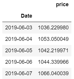
# Create a copy of two dataframes for the trading strategies
df_mg = df.copy()
df_anti_mg = df.copy()
「簡單的馬丁格爾策略」
馬丁格爾交易策略是在虧損的交易中加倍你的交易量。
我們從AAPL的一只股票開始,在虧損的交易中把交易量或數(shù)量翻倍。構(gòu)建策略時(shí),將獲勝的交易視為比前一收盤價(jià)增加2%,將失敗的交易視為比前一收盤價(jià)減少2%。
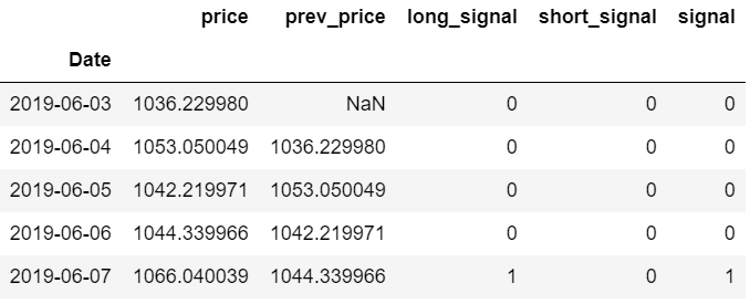
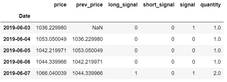
# Create column for previous price
df_mg['prev_price'] = df_mg['price'].shift(1)

# Generate buy and sell signal for price increase and decrease respectively. And create consolidated 'signal' column by addition of both buy and sell signals
df_mg['long_signal'] = np.where(df_mg['price'] > 1.02*df_mg['prev_price'], 1, 0)
df_mg['short_signal'] = np.where(df_mg['price'] < .98*df_mg['prev_price'], -1, 0)
df_mg['signal'] = df_mg['short_signal'] + df_mg['long_signal']
df_mg.head()
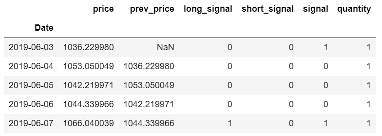
# Initialise 'quantity' column
df_mg['quantity'] = 0

# Start with 1 stock, long position
df_mg['signal'].iloc[0] = 1

# Strategy to double the trade volume or quantity on losing trades
for i in range(df_mg.shape[0]):
  if i == 0:
    df_mg['quantity'].iloc[0] = 1
  else:
    if df_mg['signal'].iloc[i] == 1:
      df_mg['quantity'].iloc[i] = df_mg['quantity'].iloc[i-1]
    if df_mg['signal'].iloc[i] == -1:
      df_mg['quantity'].iloc[i] = df_mg['quantity'].iloc[i-1]*2
    if df_mg['signal'].iloc[i] == 0:
      df_mg['quantity'].iloc[i] = df_mg['quantity'].iloc[i-1]

df_mg.head()
# Calculate returns
df_mg['returns'] = ((df_mg['price'] - df_mg['prev_price'])/ df_mg['price'])*df_mg['quantity']
# Cumulative strategy returns
df_mg['cumulative_returns'] = (df_mg.returns+1).cumprod()
# Plot cumulative returns
plt.figure(figsize=(10,5))
plt.plot(df_mg.cumulative_returns)
plt.grid()
# Define the label for the title of the figure
plt.title('Cumulative Returns for Martingale strategy', fontsize=16)
# Define the labels for x-axis and y-axis
plt.xlabel('Date', fontsize=14)
plt.ylabel('Cumulative Returns', fontsize=14)
# Define the tick size for x-axis and y-axis
plt.xticks(fontsize=12)
plt.yticks(fontsize=12)
plt.show()
# Plot position
plt.figure(figsize=(10,5))
plt.plot(df_mg.quantity)
plt.grid()

# Define the label for the title of the figure
plt.title('Position sizing', fontsize=16)

# Define the labels for x-axis and y-axis
plt.xlabel('Price', fontsize=14)
plt.ylabel('Quantity', fontsize=14)

# Define the tick size for x-axis and y-axis
plt.xticks(fontsize=12)
plt.yticks(fontsize=12)

plt.show()
注意:我們可以從上圖中注意到,交易量或數(shù)量以指數(shù)形式增加,累計(jì)收益也隨之增加。但在這種情況下,我們可能會(huì)耗盡資本來加倍倉位,從而導(dǎo)致破產(chǎn)。
「簡單的反馬丁格爾策略」
反馬丁格爾策略是在獲勝的交易中把交易量翻倍,在失敗的交易中把交易量減半。
與上述馬丁格爾策略類似,我們從AAPL的一只股票開始,在獲勝的交易中把交易量或數(shù)量增加一倍,在失敗的交易中把交易量或數(shù)量減少一半。該策略的建立是考慮到盈利的交易是2%的增長,而失敗的交易是在前一個(gè)收盤價(jià)的基礎(chǔ)上減少2%。
# This step before deciding trade size is same as the above martingale strategy
# Create column for previous price
df_anti_mg['prev_price'] = df_anti_mg['price'].shift(1)

# Generate buy and sell signal for price increase and decrease respectively. And create consolidated 'signal' column by addition of both buy and sell signals
df_anti_mg['long_signal'] = np.where(df_anti_mg['price'] > 1.02*df_anti_mg['prev_price'], 1, 0)
df_anti_mg['short_signal'] = np.where(df_anti_mg['price'] < .98*df_anti_mg['prev_price'], -1, 0)
df_anti_mg['signal'] = df_anti_mg['short_signal'] + df_anti_mg['long_signal']
df_anti_mg.head()
# Intialise 'quantity' column
df_anti_mg['quantity'] = 0

# Start with $10,000 cash long position
cash = 10000
df_anti_mg['signal'].iloc[0] = 1

# Strategy to double the trade volume or quantity on losing trades
for i in range(df_anti_mg.shape[0]):
  if i == 0:
    df_anti_mg['quantity'].iloc[0] = 1
  else:
    if df_anti_mg['signal'].iloc[i] == 1:
      df_anti_mg['quantity'].iloc[i] = df_anti_mg['quantity'].iloc[i-1]*2
    if df_anti_mg['signal'].iloc[i] == -1:
      df_anti_mg['quantity'].iloc[i] = df_anti_mg['quantity'].iloc[i-1]/2
    if df_anti_mg['signal'].iloc[i] == 0:
      df_anti_mg['quantity'].iloc[i] = df_anti_mg['quantity'].iloc[i-1]

df_anti_mg.head()
# Calculate returns
df_anti_mg['returns'] = ((df_anti_mg['price'] - df_anti_mg['prev_price'])/ df_anti_mg['prev_price'])*df_anti_mg['quantity']
# Cumulative strategy returns
df_anti_mg['cumulative_returns'] = (df_anti_mg.returns+1).cumprod()
# Plot cumulative returns
plt.figure(figsize=(10,5))
plt.plot(df_anti_mg.cumulative_returns)
plt.grid()
# Define the label for the title of the figure
plt.title('Cumulative Returns for Anti-Martingale strategy', fontsize=16)
# Define the labels for x-axis and y-axis
plt.xlabel('Date', fontsize=14)
plt.ylabel('Cumulative Returns', fontsize=14)
# Define the tick size for x-axis and y-axis
plt.xticks(fontsize=12)
plt.yticks(fontsize=12)
plt.show()
# Plot position
plt.figure(figsize=(10,5))
plt.plot(df_anti_mg.quantity)
plt.grid()

# Define the label for the title of the figure
plt.title('Position sizing', fontsize=16)

# Define the labels for x-axis and y-axis
plt.xlabel('Date', fontsize=14)
plt.ylabel('Quantity', fontsize=14)

# Define the tick size for x-axis and y-axis
plt.xticks(fontsize=12)
plt.yticks(fontsize=12)

plt.show()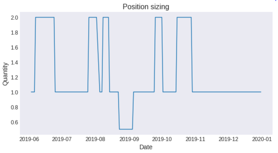
標(biāo)準(zhǔn)馬丁格爾在長期內(nèi)會(huì)導(dǎo)致高度可變的結(jié)果,因?yàn)樗赡軙?huì)遇到指數(shù)級(jí)增長的損失。而反馬丁格爾的回報(bào)分布明顯更平坦,方差更小,因?yàn)樗鼫p少了損失的風(fēng)險(xiǎn),而增加了利潤的風(fēng)險(xiǎn)。考慮到這一點(diǎn),我們看到大多數(shù)成功的交易者傾向于遵循反馬丁格爾策略,因?yàn)榕c馬丁格爾策略相比,他們被認(rèn)為在連勝期間增加投資規(guī)模的風(fēng)險(xiǎn)較小。
「總結(jié)」
在這篇文章中,我們首先通過條件期望值的概念了解了馬丁格爾的直觀含義。接下來,我們學(xué)習(xí)了馬丁格爾策略的類型。在馬丁格爾交易策略下,交易規(guī)模或數(shù)量在虧損的交易中翻倍,通過后面的盈利交易來彌補(bǔ)虧損并產(chǎn)生利潤。在反馬丁格爾交易策略中,交易規(guī)模或數(shù)量在虧損的交易中減半,在盈利的交易中翻倍。我們還了解了可能適合這兩種策略的市場條件。最后,我們用Python實(shí)現(xiàn)了馬丁格爾和反馬丁格爾交易策略。

E N D

掃描本文最下方二維碼獲取源碼和數(shù)據(jù)文件打包下載。

↓↓長按掃碼獲取完整源碼↓↓