
溫州大學(xué)《機器學(xué)習(xí)》課程代碼(三)邏輯回歸
在這一次練習(xí)中,我們將要實現(xiàn)邏輯回歸并且應(yīng)用到一個分類任務(wù)。我們還將通過將正則化加入訓(xùn)練算法,來提高算法的魯棒性,并用更復(fù)雜的情形來測試它。
代碼修改并注釋:
代碼下載:
https://github.com/fengdu78/WZU-machine-learning-course
邏輯回歸
在訓(xùn)練的初始階段,我們將要構(gòu)建一個邏輯回歸模型來預(yù)測,某個學(xué)生是否被大學(xué)錄取。設(shè)想你是大學(xué)相關(guān)部分的管理者,想通過申請學(xué)生兩次測試的評分,來決定他們是否被錄取。現(xiàn)在你擁有之前申請學(xué)生的可以用于訓(xùn)練邏輯回歸的訓(xùn)練樣本集。對于每一個訓(xùn)練樣本,你有他們兩次測試的評分和最后是被錄取的結(jié)果。為了完成這個預(yù)測任務(wù),我們準(zhǔn)備構(gòu)建一個可以基于兩次測試評分來評估錄取可能性的分類模型。
讓我們從檢查數(shù)據(jù)開始。
import numpy as np
import pandas as pd
import matplotlib.pyplot as plt
path = 'ex2data1.txt'
data = pd.read_csv(path, header=None, names=['Exam 1', 'Exam 2', 'Admitted'])
data.head()
| Exam 1 | Exam 2 | Admitted | |
|---|---|---|---|
| 0 | 34.623660 | 78.024693 | 0 |
| 1 | 30.286711 | 43.894998 | 0 |
| 2 | 35.847409 | 72.902198 | 0 |
| 3 | 60.182599 | 86.308552 | 1 |
| 4 | 79.032736 | 75.344376 | 1 |
data.shape
(100, 3)
讓我們創(chuàng)建兩個分?jǐn)?shù)的散點圖,并使用顏色編碼來可視化,如果樣本是正的(被接納)或負(fù)的(未被接納)。
positive = data[data['Admitted'].isin([1])]
negative = data[data['Admitted'].isin([0])]

fig, ax = plt.subplots(figsize=(12, 8))
ax.scatter(positive['Exam 1'],
           positive['Exam 2'],
           s=50,
           c='b',
           marker='o',
           label='Admitted')
ax.scatter(negative['Exam 1'],
           negative['Exam 2'],
           s=50,
           c='r',
           marker='x',
           label='Not Admitted')
ax.legend()
ax.set_xlabel('Exam 1 Score')
ax.set_ylabel('Exam 2 Score')
plt.show()
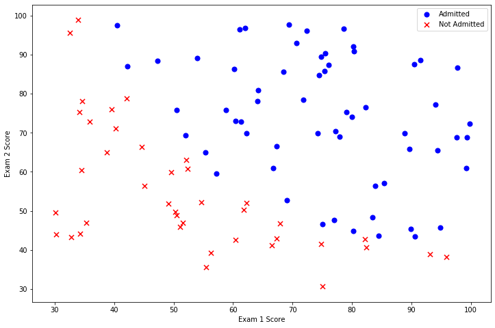
看起來在兩類間,有一個清晰的決策邊界。現(xiàn)在我們需要實現(xiàn)邏輯回歸,那樣就可以訓(xùn)練一個模型來預(yù)測結(jié)果。
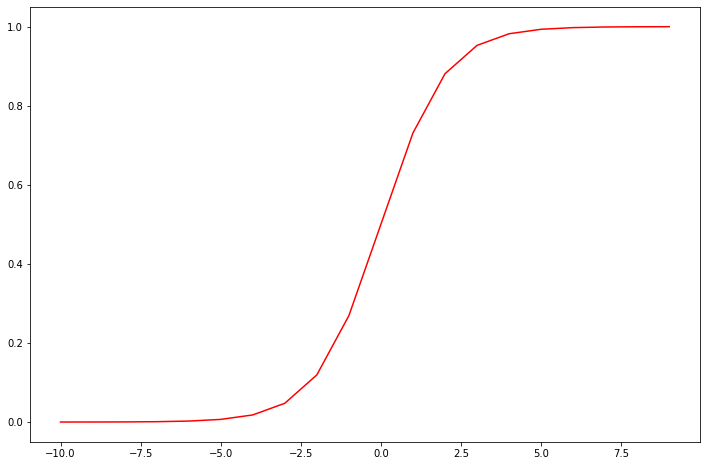
Sigmoid 函數(shù)
代表一個常用的邏輯函數(shù)(logistic function)為形函數(shù)(Sigmoid function),公式為:
合起來,我們得到邏輯回歸模型的假設(shè)函數(shù):
def sigmoid(z):
    return 1 / (1 + np.exp(-z))
讓我們做一個快速的檢查,來確保它可以工作。
nums = np.arange(-10, 10, step=1)

fig, ax = plt.subplots(figsize=(12, 8))
ax.plot(nums, sigmoid(nums), 'r')
plt.show()
棒極了!現(xiàn)在,我們需要編寫代價函數(shù)來評估結(jié)果。代價函數(shù):
def cost(w, X, y):
    w = np.matrix(w)
    X = np.matrix(X)
    y = np.matrix(y)
    first = np.multiply(-y, np.log(sigmoid(X * w.T)))
    second = np.multiply((1 - y), np.log(1 - sigmoid(X * w.T)))
    return np.sum(first - second) / (len(X))
現(xiàn)在,我們要做一些設(shè)置,和我們在練習(xí)1在線性回歸的練習(xí)很相似。
# add a ones column - this makes the matrix multiplication work out easier
data.insert(0, 'Ones', 1)

# set X (training data) and y (target variable)
cols = data.shape[1]
X = data.iloc[:, 0:cols - 1]
y = data.iloc[:, cols - 1:cols]

# convert to numpy arrays and initalize the parameter array w
X = np.array(X.values)
y = np.array(y.values)
w = np.zeros(3)
讓我們來檢查矩陣的維度來確保一切良好。
X.shape, w.shape, y.shape
((100, 3), (3,), (100, 1))
讓我們計算初始化參數(shù)的代價函數(shù)(為0)。
cost(w, X, y)
0.6931471805599453
看起來不錯,接下來,我們需要一個函數(shù)來計算我們的訓(xùn)練數(shù)據(jù)、標(biāo)簽和一些參數(shù)的梯度。
gradient descent(梯度下降)
這是批量梯度下降(batch gradient descent) 轉(zhuǎn)化為向量化計算:
def gradient(w, X, y):
    w = np.matrix(w)
    X = np.matrix(X)
    y = np.matrix(y)

    parameters = int(w.ravel().shape[1])
    grad = np.zeros(parameters)

    error = sigmoid(X * w.T) - y

    for i in range(parameters):
        term = np.multiply(error, X[:, i])
        grad[i] = np.sum(term) / len(X)

    return grad
注意,我們實際上沒有在這個函數(shù)中執(zhí)行梯度下降,我們僅僅在計算一個梯度步長。在練習(xí)中,一個稱為“fminunc”的Octave函數(shù)是用來優(yōu)化函數(shù)來計算成本和梯度參數(shù)。由于我們使用Python,我們可以用SciPy的“optimize”命名空間來做同樣的事情。
我們看看用我們的數(shù)據(jù)和初始參數(shù)為0的梯度下降法的結(jié)果。
gradient(w, X, y)
array([ -0.1 , -12.00921659, -11.26284221])
現(xiàn)在可以用SciPy's truncated newton(TNC)實現(xiàn)尋找最優(yōu)參數(shù)。
import scipy.optimize as opt
result = opt.fmin_tnc(func=cost, x0=w, fprime=gradient, args=(X, y))
result
(array([-25.16131872, 0.20623159, 0.20147149]), 36, 0)
讓我們看看在這個結(jié)論下代價函數(shù)計算結(jié)果是什么個樣子~
cost(result[0], X, y)
0.20349770158947425
接下來,我們需要編寫一個函數(shù),用我們所學(xué)的參數(shù)w來為數(shù)據(jù)集X輸出預(yù)測。然后,我們可以使用這個函數(shù)來給我們的分類器的訓(xùn)練精度打分。邏輯回歸模型的假設(shè)函數(shù):
當(dāng)大于等于0.5時,預(yù)測 y=1當(dāng)小于0.5時,預(yù)測 y=0 。
def predict(w, X):
    probability = sigmoid(X * w.T)
    return [1 if x >= 0.5 else 0 for x in probability]
w_min = np.matrix(result[0])
predictions = predict(w_min, X)
correct = [
    1 if ((a == 1 and b == 1) or (a == 0 and b == 0)) else 0
    for (a, b) in zip(predictions, y)
]
accuracy = (sum(map(int, correct)) % len(correct))
print('accuracy = {0}%'.format(accuracy))
accuracy = 89%
我們的邏輯回歸分類器預(yù)測正確,如果一個學(xué)生被錄取或沒有錄取,達(dá)到89%的精確度。不壞!記住,這是訓(xùn)練集的準(zhǔn)確性。我們沒有保持住了設(shè)置或使用交叉驗證得到的真實逼近,所以這個數(shù)字有可能高于其真實值(這個話題將在以后說明)。
正則化邏輯回歸
在訓(xùn)練的第二部分,我們將要通過加入正則項提升邏輯回歸算法。如果你對正則化有點眼生,或者喜歡這一節(jié)的方程的背景,請參考在"exercises"文件夾中的"ex2.pdf"。簡而言之,正則化是成本函數(shù)中的一個術(shù)語,它使算法更傾向于“更簡單”的模型(在這種情況下,模型將更小的系數(shù))。這個理論助于減少過擬合,提高模型的泛化能力。這樣,我們開始吧。
設(shè)想你是工廠的生產(chǎn)主管,你有一些芯片在兩次測試中的測試結(jié)果。對于這兩次測試,你想決定是否芯片要被接受或拋棄。為了幫助你做出艱難的決定,你擁有過去芯片的測試數(shù)據(jù)集,從其中你可以構(gòu)建一個邏輯回歸模型。
和第一部分很像,從數(shù)據(jù)可視化開始吧!
path = 'ex2data2.txt'
data2 = pd.read_csv(path, header=None, names=['Test 1', 'Test 2', 'Accepted'])
data2.head()
| Test 1 | Test 2 | Accepted | |
|---|---|---|---|
| 0 | 0.051267 | 0.69956 | 1 |
| 1 | -0.092742 | 0.68494 | 1 |
| 2 | -0.213710 | 0.69225 | 1 |
| 3 | -0.375000 | 0.50219 | 1 |
| 4 | -0.513250 | 0.46564 | 1 |
positive = data2[data2['Accepted'].isin([1])]
negative = data2[data2['Accepted'].isin([0])]

fig, ax = plt.subplots(figsize=(12, 8))
ax.scatter(positive['Test 1'],
           positive['Test 2'],
           s=50,
           c='b',
           marker='o',
           label='Accepted')
ax.scatter(negative['Test 1'],
           negative['Test 2'],
           s=50,
           c='r',
           marker='x',
           label='Rejected')
ax.legend()
ax.set_xlabel('Test 1 Score')
ax.set_ylabel('Test 2 Score')
plt.show()
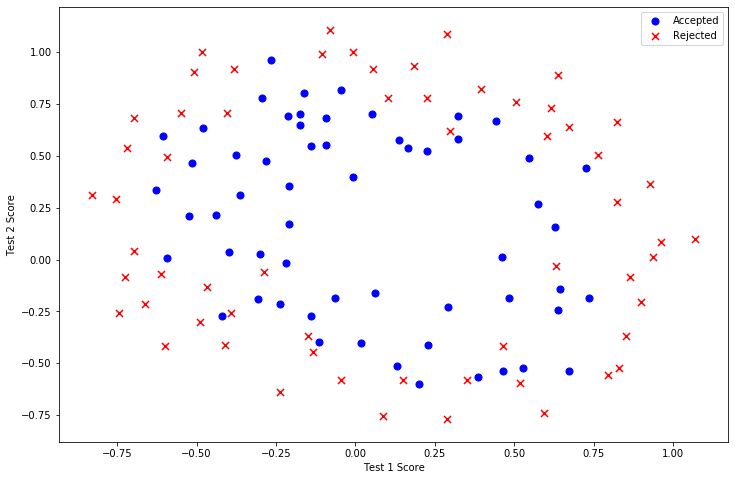
這個數(shù)據(jù)看起來可比前一次的復(fù)雜得多。特別地,你會注意到其中沒有線性決策界限,來良好的分開兩類數(shù)據(jù)。一個方法是用像邏輯回歸這樣的線性技術(shù)來構(gòu)造從原始特征的多項式中得到的特征。讓我們通過創(chuàng)建一組多項式特征入手吧。
degree = 5
x1 = data2['Test 1']
x2 = data2['Test 2']

data2.insert(3, 'Ones', 1)

for i in range(1, degree):
    for j in range(0, i):
        data2['F' + str(i) + str(j)] = np.power(x1, i-j) * np.power(x2, j)

data2.drop('Test 1', axis=1, inplace=True)
data2.drop('Test 2', axis=1, inplace=True)

data2.head()
| Accepted | Ones | F10 | F20 | F21 | F30 | F31 | F32 | F40 | F41 | F42 | F43 | |
|---|---|---|---|---|---|---|---|---|---|---|---|---|
| 0 | 1 | 1 | 0.051267 | 0.002628 | 0.035864 | 0.000135 | 0.001839 | 0.025089 | 0.000007 | 0.000094 | 0.001286 | 0.017551 |
| 1 | 1 | 1 | -0.092742 | 0.008601 | -0.063523 | -0.000798 | 0.005891 | -0.043509 | 0.000074 | -0.000546 | 0.004035 | -0.029801 |
| 2 | 1 | 1 | -0.213710 | 0.045672 | -0.147941 | -0.009761 | 0.031616 | -0.102412 | 0.002086 | -0.006757 | 0.021886 | -0.070895 |
| 3 | 1 | 1 | -0.375000 | 0.140625 | -0.188321 | -0.052734 | 0.070620 | -0.094573 | 0.019775 | -0.026483 | 0.035465 | -0.047494 |
| 4 | 1 | 1 | -0.513250 | 0.263426 | -0.238990 | -0.135203 | 0.122661 | -0.111283 | 0.069393 | -0.062956 | 0.057116 | -0.051818 |
現(xiàn)在,我們需要修改第1部分的成本和梯度函數(shù),包括正則化項。首先是成本函數(shù):
regularized cost(正則化代價函數(shù))
def costReg(w, X, y, learningRate):
    w = np.matrix(w)
    X = np.matrix(X)
    y = np.matrix(y)
    first = np.multiply(-y, np.log(sigmoid(X * w.T)))
    second = np.multiply((1 - y), np.log(1 - sigmoid(X * w.T)))
    reg = (learningRate /
           (2 * len(X))) * np.sum(np.power(w[:, 1:w.shape[1]], 2))
    return np.sum(first - second) / len(X) + reg
請注意等式中的"reg" 項。還注意到另外的一個“學(xué)習(xí)率”參數(shù)。這是一種超參數(shù),用來控制正則化項。現(xiàn)在我們需要添加正則化梯度函數(shù):
如果我們要使用梯度下降法令這個代價函數(shù)最小化,因為我們未對 進行正則化,所以梯度下降算法將分兩種情形:
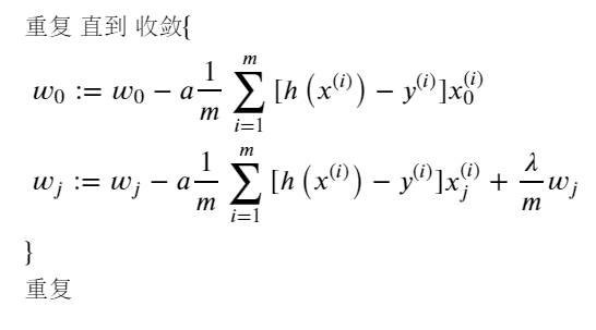
對上面的算法中 j=1,2,...,n 時的更新式子進行調(diào)整可得:
def gradientReg(w, X, y, learningRate):
    w = np.matrix(w)
    X = np.matrix(X)
    y = np.matrix(y)

    parameters = int(w.ravel().shape[1])
    grad = np.zeros(parameters)

    error = sigmoid(X * w.T) - y

    for i in range(parameters):
        term = np.multiply(error, X[:, i])

        if (i == 0):
            grad[i] = np.sum(term) / len(X)
        else:
            grad[i] = (np.sum(term) / len(X)) + (
                (learningRate / len(X)) * w[:, i])

    return grad
就像在第一部分中做的一樣,初始化變量。
# set X and y (remember from above that we moved the label to column 0)
cols = data2.shape[1]
X2 = data2.iloc[:,1:cols]
y2 = data2.iloc[:,0:1]

# convert to numpy arrays and initalize the parameter array w
X2 = np.array(X2.values)
y2 = np.array(y2.values)
w2 = np.zeros(11)
讓我們初始學(xué)習(xí)率到一個合理值。如果有必要的話(即如果懲罰太強或不夠強),我們可以之后再折騰這個。
learningRate = 1
現(xiàn)在,讓我們嘗試調(diào)用新的默認(rèn)為0的的正則化函數(shù),以確保計算工作正常。
costReg(w2, X2, y2, learningRate)
0.6931471805599454
gradientReg(w2, X2, y2, learningRate)
array([0.00847458, 0.01878809, 0.05034464, 0.01150133, 0.01835599,
       0.00732393, 0.00819244, 0.03934862, 0.00223924, 0.01286005,
       0.00309594])
現(xiàn)在我們可以使用和第一部分相同的優(yōu)化函數(shù)來計算優(yōu)化后的結(jié)果。
result2 = opt.fmin_tnc(func=costReg, x0=w2, fprime=gradientReg, args=(X2, y2, learningRate))
result2
(array([ 0.53010248,  0.29075567, -1.60725764, -0.58213819,  0.01781027,
        -0.21329508, -0.40024142, -1.37144139,  0.02264304, -0.9503358 ,
         0.0344085 ]),
 22,
 1)
最后,我們可以使用第1部分中的預(yù)測函數(shù)來查看我們的方案在訓(xùn)練數(shù)據(jù)上的準(zhǔn)確度。
w_min = np.matrix(result2[0])
predictions = predict(w_min, X2)
correct = [1 if ((a == 1 and b == 1) or (a == 0 and b == 0)) else 0 for (a, b) in zip(predictions, y2)]
accuracy = (sum(map(int, correct)) % len(correct))
print ('accuracy = {0}%'.format(accuracy))
accuracy = 78%
雖然我們實現(xiàn)了這些算法,值得注意的是,我們還可以使用高級Python庫像scikit-learn來解決這個問題。
from sklearn import linear_model#調(diào)用sklearn的線性回歸包
model = linear_model.LogisticRegression(penalty='l2', C=1.0)
model.fit(X2, y2.ravel())
LogisticRegression()
model.score(X2, y2)
0.6610169491525424
這個準(zhǔn)確度和我們剛剛實現(xiàn)的差了好多,不過請記住這個結(jié)果可以使用默認(rèn)參數(shù)下計算的結(jié)果。我們可能需要做一些參數(shù)的調(diào)整來獲得和我們之前結(jié)果相同的精確度。
參考
Prof. Andrew Ng. Machine Learning. Stanford University
往期精彩回顧
本站qq群851320808,加入微信群請掃碼: