
基于OpenCV的視頻防抖技術(shù)
點(diǎn)擊上方“小白學(xué)視覺”,選擇加"星標(biāo)"或“置頂”
重磅干貨,第一時(shí)間送達(dá)
推薦閱讀

這篇文章分享了一個(gè)視頻防抖的策略,這個(gè)方法同樣可以應(yīng)用到其他領(lǐng)域,比如常見的關(guān)鍵點(diǎn)檢測,當(dāng)使用視頻測試時(shí),效果就沒有demo那么好,此時(shí)可以考慮本文的方法去優(yōu)化。
分享這些demo并不一定所有人都會(huì)用到,但是在解決實(shí)際問題的時(shí)候,可以提供一個(gè)思路去解決問題。希望能給我一個(gè)三連,鼓勵(lì)一下哈
在這篇文章中,我們將學(xué)習(xí)如何使用OpenCV庫中的點(diǎn)特征匹配技術(shù)來實(shí)現(xiàn)一個(gè)簡單的視頻穩(wěn)定器。我們將討論算法并且會(huì)分享代碼(python和C++版),以使用這種方法在OpenCV中設(shè)計(jì)一個(gè)簡單的穩(wěn)定器。
視頻中低頻攝像機(jī)運(yùn)動(dòng)的例子
視頻防抖是指用于減少攝像機(jī)運(yùn)動(dòng)對最終視頻的影響的一系列方法。攝像機(jī)的運(yùn)動(dòng)可以是平移(比如沿著x、y、z方向上的運(yùn)動(dòng))或旋轉(zhuǎn)(偏航、俯仰、翻滾)。
視頻防抖的應(yīng)用
對視頻防抖的需求在許多領(lǐng)域都有。
這在消費(fèi)者和專業(yè)攝像中是極其重要的。因此,存在許多不同的機(jī)械、光學(xué)和算法解決方案。即使在靜態(tài)圖像拍攝中,防抖技術(shù)也可以幫助拍攝長時(shí)間曝光的手持照片。
在內(nèi)窺鏡和結(jié)腸鏡等醫(yī)療診斷應(yīng)用中,需要對視頻進(jìn)行穩(wěn)定,以確定問題的確切位置和寬度。
同樣,在軍事應(yīng)用中,無人機(jī)在偵察飛行中捕獲的視頻也需要進(jìn)行穩(wěn)定,以便定位、導(dǎo)航、目標(biāo)跟蹤等。同樣的道理也適用于機(jī)器人。
視頻防抖的不同策略
視頻防抖的方法包括機(jī)械穩(wěn)定方法、光學(xué)穩(wěn)定方法和數(shù)字穩(wěn)定方法。下面將簡要討論這些問題:
機(jī)械視頻穩(wěn)定:機(jī)械圖像穩(wěn)定系統(tǒng)使用由特殊傳感器如陀螺儀和加速度計(jì)檢測到的運(yùn)動(dòng)來移動(dòng)圖像傳感器以補(bǔ)償攝像機(jī)的運(yùn)動(dòng)。
光學(xué)視頻穩(wěn)定:在這種方法中,不是移動(dòng)整個(gè)攝像機(jī),而是通過鏡頭的移動(dòng)部分來實(shí)現(xiàn)穩(wěn)定。這種方法使用了一個(gè)可移動(dòng)的鏡頭組合,當(dāng)光通過相機(jī)的鏡頭系統(tǒng)時(shí),可以可變地調(diào)整光的路徑長度。
數(shù)字視頻穩(wěn)定:這種方法不需要特殊的傳感器來估計(jì)攝像機(jī)的運(yùn)動(dòng)。主要有三個(gè)步驟:1)運(yùn)動(dòng)估計(jì)2)運(yùn)動(dòng)平滑,3)圖像合成。第一步導(dǎo)出了兩個(gè)連續(xù)坐標(biāo)系之間的變換參數(shù)。第二步過濾不需要的運(yùn)動(dòng),在最后一步重建穩(wěn)定的視頻。
在這篇文章中,我們將學(xué)習(xí)一個(gè)快速和魯棒性好的數(shù)字視頻穩(wěn)定算法的實(shí)現(xiàn)。它是基于二維運(yùn)動(dòng)模型,其中我們應(yīng)用歐幾里得(即相似性)變換包含平移、旋轉(zhuǎn)和縮放。
OpenCV Motion Models

正如你在上面的圖片中看到的,在歐幾里得運(yùn)動(dòng)模型中,圖像中的一個(gè)正方形可以轉(zhuǎn)換為任何其他位置、大小或旋轉(zhuǎn)不同的正方形。它比仿射變換和單應(yīng)變換限制更嚴(yán)格,但對于運(yùn)動(dòng)穩(wěn)定來說足夠了,因?yàn)閿z像機(jī)在視頻連續(xù)幀之間的運(yùn)動(dòng)通常很小。
使用點(diǎn)特征匹配實(shí)現(xiàn)視頻防抖
該方法涉及跟蹤兩個(gè)連續(xù)幀之間的多個(gè)特征點(diǎn)。跟蹤特征允許我們估計(jì)幀之間的運(yùn)動(dòng)并對其進(jìn)行補(bǔ)償。
下面的流程圖顯示了基本步驟。
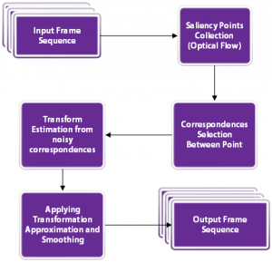
我們來看看這些步驟。
首先,讓我們完成讀取輸入視頻和寫入輸出視頻的設(shè)置。代碼中的注釋解釋每一行。
Python
# Import numpy and OpenCVimport numpy as npimport cv2# Read input videocap = cv2.VideoCapture('video.mp4')# Get frame countn_frames = int(cap.get(cv2.CAP_PROP_FRAME_COUNT))# Get width and height of video streamw = int(cap.get(cv2.CAP_PROP_FRAME_WIDTH))h = int(cap.get(cv2.CAP_PROP_FRAME_HEIGHT))# Define the codec for output videofourcc = cv2.VideoWriter_fourcc(*'MJPG')# Set up output videoout = cv2.VideoWriter('video_out.mp4', fourcc, fps, (w, h))
C++
// Read input videoVideoCapture cap("video.mp4");// Get frame countint n_frames = int(cap.get(CAP_PROP_FRAME_COUNT));// Get width and height of video streamint w = int(cap.get(CAP_PROP_FRAME_WIDTH));int h = int(cap.get(CAP_PROP_FRAME_HEIGHT));// Get frames per second (fps)double fps = cap.get(CV_CAP_PROP_FPS);// Set up output videoVideoWriter out("video_out.avi", CV_FOURCC('M','J','P','G'), fps, Size(2 * w, h));
對于視頻穩(wěn)定,我們需要捕捉視頻的兩幀,估計(jì)幀之間的運(yùn)動(dòng),最后校正運(yùn)動(dòng)。
Python
# Read first frame_, prev = cap.read()# Convert frame to grayscaleprev_gray = cv2.cvtColor(prev, cv2.COLOR_BGR2GRAY)
C++
// Define variable for storing framesMat curr, curr_gray;Mat prev, prev_gray;// Read first framecap >> prev;// Convert frame to grayscalecvtColor(prev, prev_gray, COLOR_BGR2GRAY);
這是算法中最關(guān)鍵的部分。我們將遍歷所有的幀,并找到當(dāng)前幀和前一幀之間的移動(dòng)。沒有必要知道每一個(gè)像素的運(yùn)動(dòng)。歐幾里得運(yùn)動(dòng)模型要求我們知道兩個(gè)坐標(biāo)系中兩個(gè)點(diǎn)的運(yùn)動(dòng)。但是在實(shí)際應(yīng)用中,找到50-100個(gè)點(diǎn)的運(yùn)動(dòng),然后用它們來穩(wěn)健地估計(jì)運(yùn)動(dòng)模型是一個(gè)好方法。
3.1 可用于跟蹤的優(yōu)質(zhì)特征
現(xiàn)在的問題是我們應(yīng)該選擇哪些點(diǎn)進(jìn)行跟蹤。請記住,跟蹤算法使用一個(gè)小補(bǔ)丁圍繞一個(gè)點(diǎn)來跟蹤它。這樣的跟蹤算法受到孔徑問題的困擾,如下面的視頻所述
因此,光滑的區(qū)域不利于跟蹤,而有很多角的紋理區(qū)域則比較好。幸運(yùn)的是,OpenCV有一個(gè)快速的特征檢測器,可以檢測最適合跟蹤的特性。它被稱為goodFeaturesToTrack)
3.2 Lucas-Kanade光流
一旦我們在前一幀中找到好的特征,我們就可以使用Lucas-Kanade光流算法在下一幀中跟蹤它們。
它是利用OpenCV中的calcOpticalFlowPyrLK函數(shù)實(shí)現(xiàn)的。在calcOpticalFlowPyrLK這個(gè)名字中,LK代表Lucas-Kanade,而Pyr代表金字塔。計(jì)算機(jī)視覺中的圖像金字塔是用來處理不同尺度(分辨率)的圖像的。
由于各種原因,calcOpticalFlowPyrLK可能無法計(jì)算出所有點(diǎn)的運(yùn)動(dòng)。例如,當(dāng)前幀的特征點(diǎn)可能會(huì)被下一幀的另一個(gè)對象遮擋。幸運(yùn)的是,您將在下面的代碼中看到,calcOpticalFlowPyrLK中的狀態(tài)標(biāo)志可以用來過濾掉這些值。
3.3 估計(jì)運(yùn)動(dòng)
回顧一下,在3.1步驟中,我們在前一幀中找到了一些好的特征。在步驟3.2中,我們使用光流來跟蹤特征。換句話說,我們已經(jīng)找到了特征在當(dāng)前幀中的位置,并且我們已經(jīng)知道了特征在前一幀中的位置。所以我們可以使用這兩組點(diǎn)來找到映射前一個(gè)坐標(biāo)系到當(dāng)前坐標(biāo)系的剛性(歐幾里德)變換。這是使用函數(shù)estimateRigidTransform完成的。
一旦我們估計(jì)了運(yùn)動(dòng),我們可以把它分解成x和y的平移和旋轉(zhuǎn)(角度)。我們將這些值存儲(chǔ)在一個(gè)數(shù)組中,這樣就可以平穩(wěn)地更改它們。
下面的代碼將完成步驟3.1到3.3。請務(wù)必閱讀代碼中的注釋以進(jìn)行后續(xù)操作。
Python
# Pre-define transformation-store arraytransforms = np.zeros((n_frames-1, 3), np.float32)for i in range(n_frames-2):# Detect feature points in previous frameprev_pts = cv2.goodFeaturesToTrack(prev_gray,maxCorners=200,qualityLevel=0.01,minDistance=30,blockSize=3)# Read next framecurr = cap.read()if not success:break# Convert to grayscalecurr_gray = cv2.cvtColor(curr, cv2.COLOR_BGR2GRAY)# Calculate optical flow (i.e. track feature points)status, err = cv2.calcOpticalFlowPyrLK(prev_gray, curr_gray, prev_pts, None)# Sanity checkassert prev_pts.shape == curr_pts.shape# Filter only valid pointsidx = np.where(status==1)[0]prev_pts = prev_pts[idx]curr_pts = curr_pts[idx]#Find transformation matrixm = cv2.estimateRigidTransform(prev_pts, curr_pts, fullAffine=False) #will only work with OpenCV-3 or less# Extract traslationdx = m[0,2]dy = m[1,2]# Extract rotation angleda = np.arctan2(m[1,0], m[0,0])# Store transformation= [dx,dy,da]# Move to next frameprev_gray = curr_gray: " + str(i) + "/" + str(n_frames) + " - Tracked points : " + str(len(prev_pts)))
C++
在c++實(shí)現(xiàn)中,我們首先定義一些類來幫助我們存儲(chǔ)估計(jì)的運(yùn)動(dòng)向量。下面的TransformParam類存儲(chǔ)了運(yùn)動(dòng)信息(dx -運(yùn)動(dòng)在x中,dy -運(yùn)動(dòng)在y中,da -角度變化),并提供了一個(gè)方法getTransform來將該運(yùn)動(dòng)轉(zhuǎn)換為變換矩陣。
struct TransformParam{TransformParam() {}TransformParam(double _dx, double _dy, double _da){dx = _dx;dy = _dy;da = _da;}double dx;double dy;double da; // anglevoid getTransform(Mat &T){// Reconstruct transformation matrix accordingly to new valuesT.at<double>(0,0) = cos(da);T.at<double>(0,1) = -sin(da);T.at<double>(1,0) = sin(da);T.at<double>(1,1) = cos(da);T.at<double>(0,2) = dx;T.at<double>(1,2) = dy;}};
在下面的代碼中,我們循環(huán)視頻幀并執(zhí)行步驟3.1到3.3。
// Pre-define transformation-store arrayvector <TransformParam> transforms;//Mat last_T;for(int i = 1; i < n_frames-1; i++){// Vector from previous and current feature pointsvector <Point2f> prev_pts, curr_pts;// Detect features in previous framegoodFeaturesToTrack(prev_gray, prev_pts, 200, 0.01, 30);// Read next framebool success = cap.read(curr);if(!success) break;// Convert to grayscalecvtColor(curr, curr_gray, COLOR_BGR2GRAY);// Calculate optical flow (i.e. track feature points)vector <uchar> status;vector <float> err;calcOpticalFlowPyrLK(prev_gray, curr_gray, prev_pts, curr_pts, status, err);// Filter only valid pointsauto prev_it = prev_pts.begin();auto curr_it = curr_pts.begin();for(size_t k = 0; k < status.size(); k++){if(status[k]){prev_it++;curr_it++;}else{prev_it = prev_pts.erase(prev_it);curr_it = curr_pts.erase(curr_it);}}// Find transformation matrixMat T = estimateRigidTransform(prev_pts, curr_pts, false);// In rare cases no transform is found.// We'll just use the last known good transform.if(T.data == NULL) last_T.copyTo(T);T.copyTo(last_T);// Extract traslationdouble dx = T.at<double>(0,2);double dy = T.at<double>(1,2);// Extract rotation angledouble da = atan2(T.at<double>(1,0), T.at<double>(0,0));// Store transformationtransforms.push_back(TransformParam(dx, dy, da));// Move to next framecurr_gray.copyTo(prev_gray);cout << "Frame: " << i << "/" << n_frames << " - Tracked points : " << prev_pts.size() << endl;}
在前面的步驟中,我們估計(jì)幀之間的運(yùn)動(dòng)并將它們存儲(chǔ)在一個(gè)數(shù)組中。我們現(xiàn)在需要通過疊加上一步估計(jì)的微分運(yùn)動(dòng)來找到運(yùn)動(dòng)軌跡。
步驟4.1:軌跡計(jì)算
在這一步,我們將增加運(yùn)動(dòng)之間的幀來計(jì)算軌跡。我們的最終目標(biāo)是平滑這條軌跡。
Python 在Python中,可以很容易地使用numpy中的cumsum(累計(jì)和)來實(shí)現(xiàn)。
# Compute trajectory using cumulative sum of transformationstrajectory = np.cumsum(transforms, axis=0
C++
在c++中,我們定義了一個(gè)名為Trajectory的結(jié)構(gòu)體來存儲(chǔ)轉(zhuǎn)換參數(shù)的累積和。
struct Trajectory{Trajectory() {}Trajectory(double _x, double _y, double _a) {x = _x;y = _y;a = _a;}double x;double y;double a; // angle};
C我們還定義了一個(gè)函數(shù)cumsum,它接受一個(gè)TransformParams 向量,并通過執(zhí)行微分運(yùn)動(dòng)dx、dy和da(角度)的累積和返回軌跡。
vector<Trajectory> cumsum(vector<TransformParam> &transforms){vector <Trajectory> trajectory; // trajectory at all frames// Accumulated frame to frame transformdouble a = 0;double x = 0;double y = 0;for(size_t i=0; i < transforms.size(); i++){x += transforms[i].dx;y += transforms[i].dy;a += transforms[i].da;trajectory.push_back(Trajectory(x,y,a));}return trajectory;}
步驟4.2:計(jì)算平滑軌跡
在上一步中,我們計(jì)算了運(yùn)動(dòng)軌跡。所以我們有三條曲線來顯示運(yùn)動(dòng)(x, y,和角度)如何隨時(shí)間變化。
在這一步,我們將展示如何平滑這三條曲線。
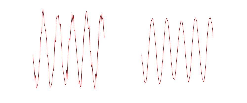
平滑任何曲線最簡單的方法是使用移動(dòng)平均濾波器(moving average filter)。顧名思義,移動(dòng)平均過濾器將函數(shù)在某一點(diǎn)上的值替換為由窗口定義的其相鄰函數(shù)的平均值。讓我們看一個(gè)例子。
假設(shè)我們在數(shù)組c中存儲(chǔ)了一條曲線,那么曲線上的點(diǎn)是c[0]…c[n-1]。設(shè)f是我們通過寬度為5的移動(dòng)平均濾波器過濾c得到的平滑曲線。
該曲線的k^{th}元素使用

如您所見,平滑曲線的值是噪聲曲線在一個(gè)小窗口上的平均值。下圖顯示了左邊的噪點(diǎn)曲線的例子,使用右邊的尺度為5 濾波器進(jìn)行平滑。
Python
在Python實(shí)現(xiàn)中,我們定義了一個(gè)移動(dòng)平均濾波器,它接受任何曲線(即1-D的數(shù)字)作為輸入,并返回曲線的平滑版本。
def movingAverage(curve, radius):window_size = 2 * radius + 1# Define the filterf = np.ones(window_size)/window_size# Add padding to the boundariescurve_pad = np.lib.pad(curve, (radius, radius), 'edge')# Apply convolutioncurve_smoothed = np.convolve(curve_pad, f, mode='same')# Remove paddingcurve_smoothed = curve_smoothed[radius:-radius]# return smoothed curvereturn curve_smoothed
我們還定義了一個(gè)函數(shù),它接受軌跡并對這三個(gè)部分進(jìn)行平滑處理。
def smooth(trajectory):smoothed_trajectory = np.copy(trajectory)# Filter the x, y and angle curvesfor i in range(3):smoothed_trajectory[:,i] = movingAverage(trajectory[:,i], radius=SMOOTHING_RADIUS)return smoothed_trajectory
# Compute trajectory using cumulative sum of transformationstrajectory = np.cumsum(transforms, axis=0)
C++
在c++版本中,我們定義了一個(gè)名為smooth的函數(shù),用于計(jì)算平滑移動(dòng)平均軌跡。
vector <Trajectory> smooth(vector <Trajectory>& trajectory, int radius){vector <Trajectory> smoothed_trajectory;for(size_t i=0; i < trajectory.size(); i++) {double sum_x = 0;double sum_y = 0;double sum_a = 0;int count = 0;for(int j=-radius; j <= radius; j++) { if(i+j >= 0 && i+j < trajectory.size()) {sum_x += trajectory[i+j].x;sum_y += trajectory[i+j].y;sum_a += trajectory[i+j].a;count++;}}double avg_a = sum_a / count;double avg_x = sum_x / count;double avg_y = sum_y / count;smoothed_trajectory.push_back(Trajectory(avg_x, avg_y, avg_a));}return smoothed_trajectory;}
我們在主函數(shù)中使用它
// Smooth trajectory using moving average filtervector <Trajectory> smoothed_trajectory = smooth(trajectory, SMOOTHING_RADIUS);
步驟4.3:計(jì)算平滑變換
到目前為止,我們已經(jīng)得到了一個(gè)平滑的軌跡。在這一步,我們將使用平滑的軌跡來獲得平滑的變換,可以應(yīng)用到視頻的幀來穩(wěn)定它。
這是通過找到平滑軌跡和原始軌跡之間的差異,并將這些差異加回到原始的變換中來完成的。
Python
# Calculate difference in smoothed_trajectory and trajectorydifference = smoothed_trajectory - trajectory# Calculate newer transformation arraytransforms_smooth = transforms + difference
C++
vectortransforms_smooth; for(size_t i=0; i < transforms.size(); i++){// Calculate difference in smoothed_trajectory and trajectorydouble diff_x = smoothed_trajectory[i].x - trajectory[i].x;double diff_y = smoothed_trajectory[i].y - trajectory[i].y;double diff_a = smoothed_trajectory[i].a - trajectory[i].a;// Calculate newer transformation arraydouble dx = transforms[i].dx + diff_x;double dy = transforms[i].dy + diff_y;double da = transforms[i].da + diff_a;transforms_smooth.push_back(TransformParam(dx, dy, da));}
差不多做完了。現(xiàn)在我們所需要做的就是循環(huán)幀并應(yīng)用我們剛剛計(jì)算的變換。
如果我們有一個(gè)指定為(x, y, \theta),的運(yùn)動(dòng),對應(yīng)的變換矩陣是

請閱讀代碼中的注釋以進(jìn)行后續(xù)操作。
Python
# Reset stream to first frame0)# Write n_frames-1 transformed framesfor i in range(n_frames-2):# Read next frameframe = cap.read()if not success:break# Extract transformations from the new transformation arraydx = transforms_smooth[i,0]dy = transforms_smooth[i,1]da = transforms_smooth[i,2]# Reconstruct transformation matrix accordingly to new valuesm = np.zeros((2,3), np.float32)= np.cos(da)= -np.sin(da)= np.sin(da)= np.cos(da)= dx= dy# Apply affine wrapping to the given frameframe_stabilized = cv2.warpAffine(frame, m, (w,h))# Fix border artifactsframe_stabilized = fixBorder(frame_stabilized)# Write the frame to the fileframe_out = cv2.hconcat([frame, frame_stabilized])# If the image is too big, resize it.> 1920):frame_out = cv2.resize(frame_out, (frame_out.shape[1]/2, frame_out.shape[0]/2));and After", frame_out)cv2.waitKey(10)out.write(frame_out)
C++
cap.set(CV_CAP_PROP_POS_FRAMES, 1);Mat T(2,3,CV_64F);Mat frame, frame_stabilized, frame_out;for( int i = 0; i < n_frames-1; i++) { bool success = cap.read(frame); if(!success) break; // Extract transform from translation and rotation angle. transforms_smooth[i].getTransform(T); // Apply affine wrapping to the given frame warpAffine(frame, frame_stabilized, T, frame.size()); // Scale image to remove black border artifact fixBorder(frame_stabilized); // Now draw the original and stabilised side by side for coolness hconcat(frame, frame_stabilized, frame_out); // If the image is too big, resize it. if(frame_out.cols > 1920){resize(frame_out, frame_out, Size(frame_out.cols/2, frame_out.rows/2));}imshow("Before and After", frame_out);out.write(frame_out);waitKey(10);}
步驟5.1:修復(fù)邊界偽影
當(dāng)我們穩(wěn)定一個(gè)視頻,我們可能會(huì)看到一些黑色的邊界偽影。這是意料之中的,因?yàn)闉榱朔€(wěn)定視頻,幀可能不得不縮小大小。
我們可以通過將視頻的中心縮小一小部分(例如4%)來緩解這個(gè)問題。
下面的fixBorder函數(shù)顯示了實(shí)現(xiàn)。我們使用getRotationMatrix2D,因?yàn)樗诓灰苿?dòng)圖像中心的情況下縮放和旋轉(zhuǎn)圖像。我們所需要做的就是調(diào)用這個(gè)函數(shù)時(shí),旋轉(zhuǎn)為0,縮放為1.04(也就是提升4%)。
Python
def fixBorder(frame):s = frame.shape# Scale the image 4% without moving the centerT = cv2.getRotationMatrix2D((s[1]/2, s[0]/2), 0, 1.04)frame = cv2.warpAffine(frame, T, (s[1], s[0]))return frame
C++
void fixBorder(Mat &frame_stabilized){Mat T = getRotationvoid fixBorder(Mat &frame_stabilized){Mat T = getRotationMatrix2D(Point2f(frame_stabilized.cols/2, frame_stabilized.rows/2), 0, 1.04);warpAffine(frame_stabilized, frame_stabilized, T, frame_stabilized.size());}Matrix2D(Point2f(frame_stabilized.cols/2, frame_stabilized.rows/2), 0, 1.04);warpAffine(frame_stabilized, frame_stabilized, T, frame_stabilized.size());}
結(jié)果:
我們分享的視頻防抖代碼的結(jié)果如上所示。我們的目標(biāo)是顯著減少運(yùn)動(dòng),但不是完全消除它。
我們留給讀者去思考如何修改代碼來完全消除幀之間的移動(dòng)。如果你試圖消除所有的相機(jī)運(yùn)動(dòng),會(huì)有什么副作用?
目前的方法只適用于固定長度的視頻,而不適用于實(shí)時(shí)feed。我們不得不對這個(gè)方法進(jìn)行大量修改,以獲得實(shí)時(shí)視頻輸出,這超出了本文的范圍,但這是可以實(shí)現(xiàn)的,更多的信息可以在這里找到。
https://abhitronix.github.io/2018/11/30/humanoid-AEAM-3/
優(yōu)點(diǎn)和缺點(diǎn)
優(yōu)點(diǎn)
這種方法對低頻運(yùn)動(dòng)(較慢的振動(dòng))具有良好的穩(wěn)定性。這種方法內(nèi)存消耗低,因此非常適合嵌入式設(shè)備(如樹莓派)。這種方法對視頻縮放抖動(dòng)有很好的效果。
缺點(diǎn)
這種方法對高頻擾動(dòng)的抵抗效果很差。如果有一個(gè)嚴(yán)重的運(yùn)動(dòng)模糊,特征跟蹤將失敗,結(jié)果將不是最佳的。這種方法也不適用于滾動(dòng)快門失真。
References:
Example video and Code reference from Nghia Ho’s?post
http://nghiaho.com/uploads/code/videostab.cpp
Various References, data, and image from my?website
https://abhitronix.github.io/
https://www.learnopencv.com/video-stabilization-using-point-feature-matching-in-opencv/
交流群
歡迎加入公眾號(hào)讀者群一起和同行交流,目前有SLAM、三維視覺、傳感器、自動(dòng)駕駛、計(jì)算攝影、檢測、分割、識(shí)別、醫(yī)學(xué)影像、GAN、算法競賽等微信群(以后會(huì)逐漸細(xì)分),請掃描下面微信號(hào)加群,備注:”昵稱+學(xué)校/公司+研究方向“,例如:”張三?+?上海交大?+?視覺SLAM“。請按照格式備注,否則不予通過。添加成功后會(huì)根據(jù)研究方向邀請進(jìn)入相關(guān)微信群。請勿在群內(nèi)發(fā)送廣告,否則會(huì)請出群,謝謝理解~