↓推薦關(guān)注↓

本文主要分析時(shí)間序列的趨勢(shì)和季節(jié)性，分解時(shí)間序列，實(shí)現(xiàn)預(yù)測(cè)模型。

時(shí)間序列預(yù)測(cè)是基于時(shí)間數(shù)據(jù)進(jìn)行預(yù)測(cè)的任務(wù)。它包括建立模型來進(jìn)行觀測(cè)，并在諸如天氣、工程、經(jīng)濟(jì)、金融或商業(yè)預(yù)測(cè)等應(yīng)用中推動(dòng)未來的決策。

本文主要介紹時(shí)間序列預(yù)測(cè)并描述任何時(shí)間序列的兩種主要模式(趨勢(shì)和季節(jié)性)。并基于這些模式對(duì)時(shí)間序列進(jìn)行分解。最后使用一個(gè)被稱為Holt-Winters季節(jié)方法的預(yù)測(cè)模型，來預(yù)測(cè)有趨勢(shì)和/或季節(jié)成分的時(shí)間序列數(shù)據(jù)。

為了涵蓋所有這些內(nèi)容，我們將使用一個(gè)時(shí)間序列數(shù)據(jù)集，包括1981年至1991年期間墨爾本(澳大利亞)的溫度。這個(gè)數(shù)據(jù)集可以從這個(gè)Kaggle下載，也可以在公眾號(hào)：Python學(xué)習(xí)與數(shù)據(jù)挖掘，后臺(tái)回復(fù)【墨爾本】下載，其中包含本文的數(shù)據(jù)和代碼。該數(shù)據(jù)集由澳大利亞政府氣象局托管，并根據(jù)該局的“默認(rèn)使用條款”(Open Access Licence)獲得許可。

導(dǎo)入庫和數(shù)據(jù)

首先，導(dǎo)入運(yùn)行代碼所需的下列庫。除了最典型的庫之外，該代碼還基于statsmomodels庫提供的函數(shù)，該庫提供了用于估計(jì)許多不同統(tǒng)計(jì)模型的類和函數(shù)，如統(tǒng)計(jì)測(cè)試和預(yù)測(cè)模型。

from datetime import datetime, timedelta
import matplotlib.pyplot as plt
import numpy as np
import pandas as pd
import statsmodels.api as sm
from statsmodels.tsa.stattools import adfuller, kpss
from statsmodels.tsa.api import ExponentialSmoothing
%matplotlib inline

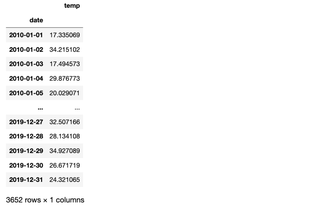
下面是導(dǎo)入數(shù)據(jù)的代碼。數(shù)據(jù)由兩列組成，一列是日期，另一列是1981年至1991年間墨爾本(澳大利亞)的溫度。

# date
numdays = 365*10 + 2
base = '2010-01-01'
base = datetime.strptime(base, '%Y-%m-%d')
date_list = [base + timedelta(days=x) for x in range(numdays)]
date_list = np.array(date_list)
print(len(date_list), date_list[0], date_list[-1])

# temp
x = np.linspace(-np.pi, np.pi, 365)
temp_year = (np.sin(x) + 1.0) * 15
x = np.linspace(-np.pi, np.pi, 366)
temp_leap_year = (np.sin(x) + 1.0)
temp_s = []
for i in range(2010, 2020):
    if i == 2010:
        temp_s = temp_year + np.random.rand(365) * 20
    elif i in [2012, 2016]:
        temp_s = np.concatenate((temp_s, temp_leap_year * 15 + np.random.rand(366) * 20 + i % 2010))
    else:
        temp_s = np.concatenate((temp_s, temp_year + np.random.rand(365) * 20 + i % 2010))
print(len(temp_s))

# df
data = np.concatenate((date_list.reshape(-1, 1), temp_s.reshape(-1, 1)), axis=1)
df_orig = pd.DataFrame(data, columns=['date', 'temp'])
df_orig['date'] =  pd.to_datetime(df_orig['date'], format='%Y-%m-%d')
df = df_orig.set_index('date')
df.sort_index(inplace=True)
df

可視化數(shù)據(jù)集

在我們開始分析時(shí)間序列的模式之前，讓我們將每個(gè)垂直虛線對(duì)應(yīng)于一年開始的數(shù)據(jù)可視化。

ax = df_orig.plot(x='date', y='temp', figsize=(12,6))
xcoords = ['2010-01-01', '2011-01-01', '2012-01-01', '2013-01-01', '2014-01-01',
           '2015-01-01', '2016-01-01', '2017-01-01', '2018-01-01', '2019-01-01']
for xc in xcoords:
    plt.axvline(x=xc, color='black', linestyle='--')
ax.set_ylabel('temperature')

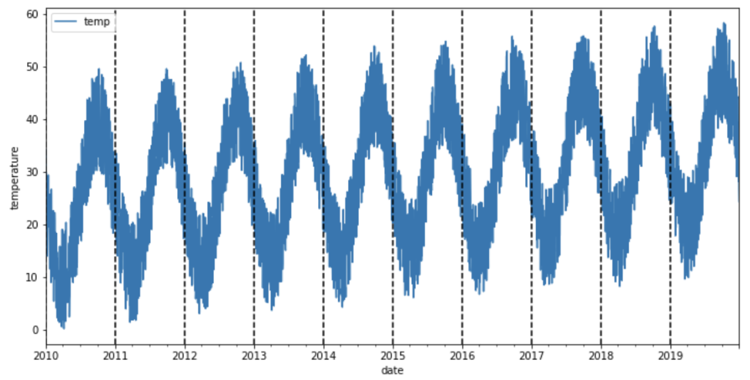
在進(jìn)入下一節(jié)之前，讓我們花點(diǎn)時(shí)間看一下數(shù)據(jù)。這些數(shù)據(jù)似乎有一個(gè)季節(jié)性的變化，冬季溫度上升，夏季溫度下降(南半球)。而且氣溫似乎不會(huì)隨著時(shí)間的推移而增加，因?yàn)闊o論哪一年的平均氣溫都是相同的。

時(shí)間序列模式

時(shí)間序列預(yù)測(cè)模型使用數(shù)學(xué)方程(s)在一系列歷史數(shù)據(jù)中找到模式。然后使用這些方程將數(shù)據(jù)[中的歷史時(shí)間模式投射到未來。

有四種類型的時(shí)間序列模式:

趨勢(shì):數(shù)據(jù)的長期增減。趨勢(shì)可以是任何函數(shù)，如線性或指數(shù)，并可以隨時(shí)間改變方向。

季節(jié)性:以固定的頻率(一天中的小時(shí)、星期、月、年等)在系列中重復(fù)的周期。季節(jié)模式存在一個(gè)固定的已知周期

周期性:當(dāng)數(shù)據(jù)漲跌時(shí)發(fā)生，但沒有固定的頻率和持續(xù)時(shí)間，例如由經(jīng)濟(jì)狀況引起。

噪音:系列中的隨機(jī)變化。

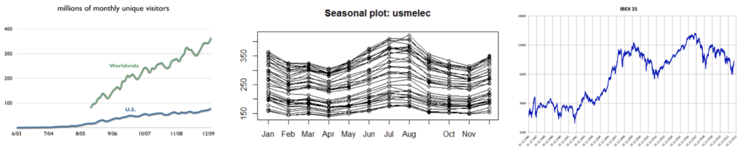
大多數(shù)時(shí)間序列數(shù)據(jù)將包含一個(gè)或多個(gè)模式，但可能不是全部。這里有一些例子，我們可以識(shí)別這些時(shí)間序列模式:

維基百科年度受眾(左圖):在這張圖中，我們可以確定一個(gè)增加的趨勢(shì)，受眾每年線性增加。

美國用電量季節(jié)性圖(中圖):每條線對(duì)應(yīng)的是一年，因此我們可以觀察到每年的用電量重復(fù)出現(xiàn)的季節(jié)性。

ibex35的日收盤價(jià)(右圖):這個(gè)時(shí)間序列隨著時(shí)間的推移有一個(gè)增加的趨勢(shì)，以及一個(gè)周期性的模式，因?yàn)橛幸恍r(shí)期ibex35由于經(jīng)濟(jì)原因而下降。

圖2 從左至右，維基百科的年度受眾，美國用電量的季節(jié)性圖，IBEX 35日關(guān)閉次數(shù)

如果我們假設(shè)對(duì)這些模式進(jìn)行加法分解，我們可以這樣寫:

Y[t] = t [t] + S[t] + e[t]

其中Y[t]為數(shù)據(jù)，t [t]為趨勢(shì)周期分量，S[t]為季節(jié)分量，e[t]為噪聲，t為時(shí)間周期。

另一方面，乘法分解可以寫成:

Y[t] = t [t] *S[t] *e[t]

當(dāng)季節(jié)波動(dòng)不隨時(shí)間序列水平變化時(shí)，加法分解是最合適的方法。相反，當(dāng)季節(jié)成分的變化與時(shí)間序列水平成正比時(shí)，則采用乘法分解更為合適。

分解數(shù)據(jù)

平穩(wěn)時(shí)間序列被定義為其不依賴于觀察到該序列的時(shí)間。因此具有趨勢(shì)或季節(jié)性的時(shí)間序列不是平穩(wěn)的，而白噪聲序列是平穩(wěn)的。從數(shù)學(xué)意義上講，如果一個(gè)時(shí)間序列的均值和方差不變，且協(xié)方差與時(shí)間無關(guān)，那么這個(gè)時(shí)間序列就是平穩(wěn)的。有不同的例子來比較平穩(wěn)和非平穩(wěn)時(shí)間序列。一般來說，平穩(wěn)時(shí)間序列不會(huì)有長期可預(yù)測(cè)的模式。

為什么穩(wěn)定性很重要呢?

平穩(wěn)性已經(jīng)成為時(shí)間序列分析中許多實(shí)踐和工具的常見假設(shè)。其中包括趨勢(shì)估計(jì)、預(yù)測(cè)和因果推斷等。因此，在許多情況下，需要確定數(shù)據(jù)是否是由固定過程生成的，并將其轉(zhuǎn)換為具有該過程生成的樣本的屬性。

如何檢驗(yàn)時(shí)間序列的平穩(wěn)性呢?

我們可以用兩種方法來檢驗(yàn)。一方面，我們可以通過檢查時(shí)間序列的均值和方差來手動(dòng)檢查。另一方面，我們可以使用測(cè)試函數(shù)來評(píng)估平穩(wěn)性。

有些情況可能會(huì)讓人感到困惑。例如一個(gè)沒有趨勢(shì)和季節(jié)性但具有周期行為的時(shí)間序列是平穩(wěn)的，因?yàn)橹芷诘拈L度不是固定的。

查看趨勢(shì)

為了分析時(shí)間序列的趨勢(shì)，我們首先使用有30天窗口的滾動(dòng)均值方法分析隨時(shí)間推移的平均值。

def analyze_stationarity(timeseries, title):
    fig, ax = plt.subplots(2, 1, figsize=(16, 8))

    rolmean = pd.Series(timeseries).rolling(window=30).mean() 
    rolstd = pd.Series(timeseries).rolling(window=30).std()
    ax[0].plot(timeseries, label= title)
    ax[0].plot(rolmean, label='rolling mean');
    ax[0].plot(rolstd, label='rolling std (x10)');
    ax[0].set_title('30-day window')
    ax[0].legend()
 
    rolmean = pd.Series(timeseries).rolling(window=365).mean() 
    rolstd = pd.Series(timeseries).rolling(window=365).std()
    ax[1].plot(timeseries, label= title)
    ax[1].plot(rolmean, label='rolling mean');
    ax[1].plot(rolstd, label='rolling std (x10)');
    ax[1].set_title('365-day window')
 
pd.options.display.float_format = '{:.8f}'.format
analyze_stationarity(df['temp'], 'raw data')
    ax[1].legend()

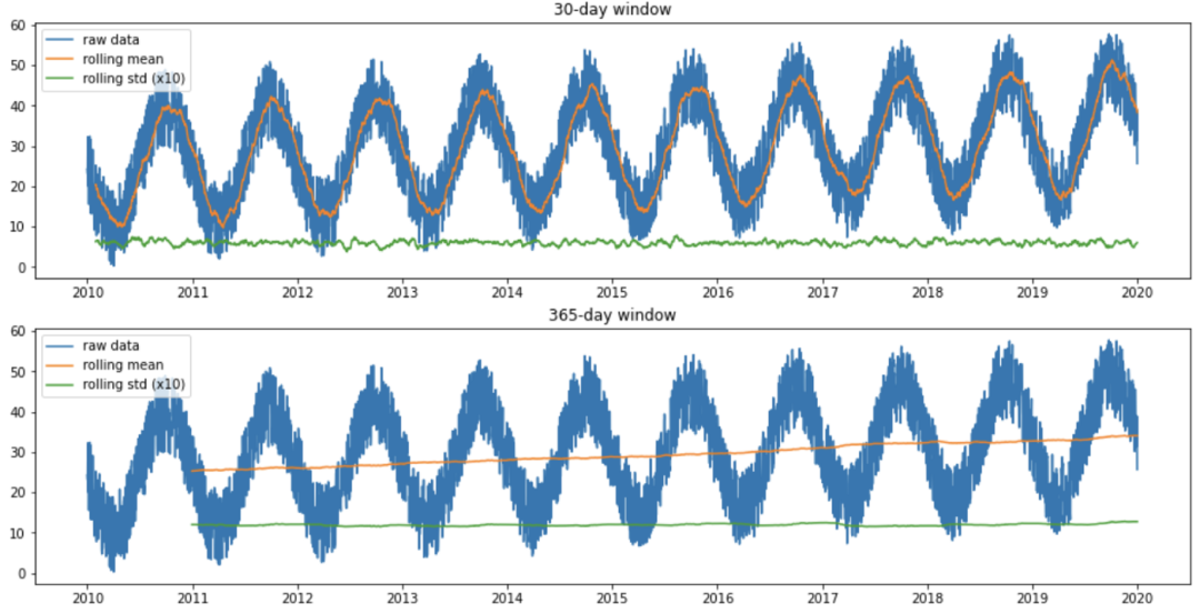
在上圖中，我們可以看到使用30天窗口時(shí)滾動(dòng)均值是如何隨時(shí)間波動(dòng)的，這是由數(shù)據(jù)的季節(jié)性模式引起的。此外，當(dāng)使用365天窗口時(shí)，滾動(dòng)平均值隨時(shí)間增加，表明隨時(shí)間略有增加的趨勢(shì)。

這也可以通過一些測(cè)試來評(píng)估，如Dickey-Fuller (ADF)和Kwiatkowski, Phillips, Schmidt和Shin (KPSS):

ADF檢驗(yàn)的結(jié)果(p值低于0.05)表明，存在的原假設(shè)可以在95%的置信水平上被拒絕。因此，如果p值低于0.05，則時(shí)間序列是平穩(wěn)的。

def ADF_test(timeseries):
    print("Results of Dickey-Fuller Test:")
    dftest = adfuller(timeseries, autolag="AIC")
    dfoutput = pd.Series(
        dftest[0:4],
        index=[
            "Test Statistic",
            "p-value",
            "Lags Used",
            "Number of Observations Used",
        ],
    )
    for key, value in dftest[4].items():
        dfoutput["Critical Value (%s)" % key] = value
    print(dfoutput)

ADF_test(df)

Results of Dickey-Fuller Test:
Test Statistic                  -3.69171446
p-value                          0.00423122
Lags Used                       30.00000000
Number of Observations Used   3621.00000000
Critical Value (1%)             -3.43215722
Critical Value (5%)             -2.86233853
Critical Value (10%)            -2.56719507
dtype: float64

KPSS檢驗(yàn)的結(jié)果(p值高于0.05)表明，在95%的置信水平下，不能拒絕的零假設(shè)。因此如果p值低于0.05，則時(shí)間序列不是平穩(wěn)的。

def KPSS_test(timeseries):
    print("Results of KPSS Test:")
    kpsstest = kpss(timeseries.dropna(), regression="c", nlags="auto")    
    kpss_output = pd.Series(
        kpsstest[0:3], index=["Test Statistic", "p-value", "Lags Used"]
    )
    for key, value in kpsstest[3].items():
        kpss_output["Critical Value (%s)" % key] = value
    print(kpss_output)

KPSS_test(df)

Results of KPSS Test:
Test Statistic           1.04843270
p-value                  0.01000000
Lags Used               37.00000000
Critical Value (10%)     0.34700000
Critical Value (5%)      0.46300000
Critical Value (2.5%)    0.57400000
Critical Value (1%)      0.73900000
dtype: float64

雖然這些檢驗(yàn)似乎是為了檢查數(shù)據(jù)的平穩(wěn)性，但這些檢驗(yàn)對(duì)于分析時(shí)間序列的趨勢(shì)而不是季節(jié)性是有用的。

統(tǒng)計(jì)結(jié)果還顯示了時(shí)間序列的平穩(wěn)性的影響。雖然兩個(gè)檢驗(yàn)的零假設(shè)是相反的。ADF檢驗(yàn)表明時(shí)間序列是平穩(wěn)的(p值> 0.05)，而KPSS檢驗(yàn)表明時(shí)間序列不是平穩(wěn)的(p值> 0.05)。但這個(gè)數(shù)據(jù)集創(chuàng)建時(shí)帶有輕微的趨勢(shì)，因此結(jié)果表明，KPSS測(cè)試對(duì)于分析這個(gè)數(shù)據(jù)集更準(zhǔn)確。

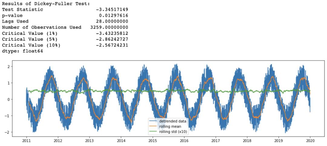
為了減少數(shù)據(jù)集的趨勢(shì)，我們可以使用以下方法消除趨勢(shì):

df_detrend = (df - df.rolling(window=365).mean()) / df.rolling(window=365).std()

analyze_stationarity(df_detrend['temp'].dropna(), 'detrended data')
ADF_test(df_detrend.dropna())

圖4 對(duì)時(shí)間序列去趨勢(shì)后的滾動(dòng)均值和標(biāo)準(zhǔn)差

檢查季節(jié)性

正如在之前從滑動(dòng)窗口中觀察到的，在我們的時(shí)間序列中有一個(gè)季節(jié)模式。因此應(yīng)該采用差分方法來去除時(shí)間序列中潛在的季節(jié)或周期模式。由于樣本數(shù)據(jù)集具有12個(gè)月的季節(jié)性，我使用了365個(gè)滯后差值:

df_365lag =  df - df.shift(365)

analyze_stationarity(df_365lag['temp'].dropna(), '12 lag differenced data')
ADF_test(df_365lag.dropna())

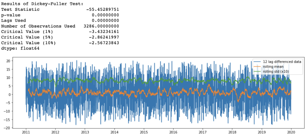
圖5 對(duì)時(shí)間序列進(jìn)行差分后的滾動(dòng)均值和標(biāo)準(zhǔn)差

現(xiàn)在，滑動(dòng)均值和標(biāo)準(zhǔn)差隨著時(shí)間的推移或多或少保持不變，所以我們有一個(gè)平穩(wěn)的時(shí)間序列。

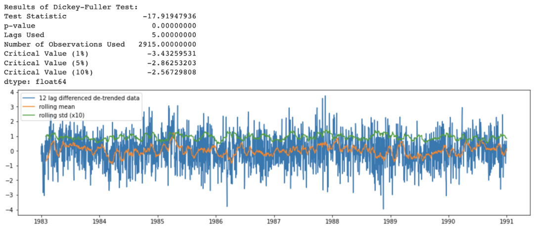
上面方法合在一起的代碼如下：

df_365lag_detrend =  df_detrend - df_detrend.shift(365)

analyze_stationarity(df_365lag_detrend['temp'].dropna(), '12 lag differenced de-trended data')
ADF_test(df_365lag_detrend.dropna())

圖6 對(duì)時(shí)間序列進(jìn)行去趨勢(shì)和差分后的滾動(dòng)均值和標(biāo)準(zhǔn)差

分解模式

基于上述模式的分解可以通過' statmodels '包中的一個(gè)有用的Python函數(shù)seasonal_decomposition來實(shí)現(xiàn):

def seasonal_decompose (df):
    decomposition = sm.tsa.seasonal_decompose(df, model='additive', freq=365)
 
    trend = decomposition.trend
    seasonal = decomposition.seasonal
    residual = decomposition.resid
 
    fig = decomposition.plot()
    fig.set_size_inches(14, 7)
    plt.show()
 
    return trend, seasonal, residual
 
seasonal_decompose(df)

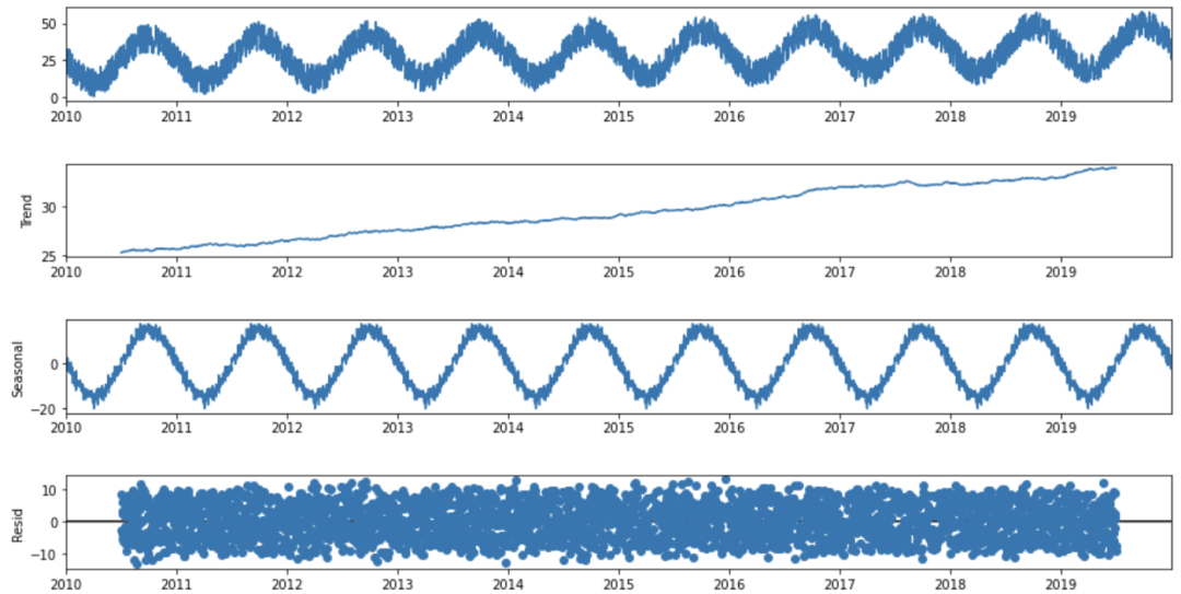
在看了分解圖的四個(gè)部分后，可以說，在我們的時(shí)間序列中有很強(qiáng)的年度季節(jié)性成分，以及隨時(shí)間推移的增加趨勢(shì)模式。

時(shí)序建模

時(shí)間序列數(shù)據(jù)的適當(dāng)模型將取決于數(shù)據(jù)的特定特征，例如，數(shù)據(jù)集是否具有總體趨勢(shì)或季節(jié)性。請(qǐng)務(wù)必選擇最適數(shù)據(jù)的模型。

我們可以使用下面這些模型：

Autoregression (AR)
Moving Average (MA)
Autoregressive Moving Average (ARMA)
Autoregressive Integrated Moving Average (ARIMA)
Seasonal Autoregressive Integrated Moving-Average (SARIMA)
Seasonal Autoregressive Integrated Moving-Average with Exogenous Regressors (SARIMAX)
Vector Autoregression (VAR)
Vector Autoregression Moving-Average (VARMA)
Vector Autoregression Moving-Average with Exogenous Regressors (VARMAX)
Simple Exponential Smoothing (SES)
Holt Winter’s Exponential Smoothing (HWES)

由于我們的數(shù)據(jù)中存在季節(jié)性，因此選擇HWES，因?yàn)樗m用于具有趨勢(shì)和/或季節(jié)成分的時(shí)間序列數(shù)據(jù)。

這種方法使用指數(shù)平滑來編碼大量的過去的值，并使用它們來預(yù)測(cè)現(xiàn)在和未來的“典型”值。指數(shù)平滑指的是使用指數(shù)加權(quán)移動(dòng)平均(EWMA)“平滑”一個(gè)時(shí)間序列。

在實(shí)現(xiàn)它之前，讓我們創(chuàng)建訓(xùn)練和測(cè)試數(shù)據(jù)集:

y = df['temp'].astype(float)
y_to_train = y[:'2017-12-31']
y_to_val = y['2018-01-01':]
predict_date = len(y) - len(y[:'2017-12-31'])

下面是使用均方根誤差(RMSE)作為評(píng)估模型誤差的度量的實(shí)現(xiàn)。

def holt_win_sea(y, y_to_train, y_to_test, seasonal_period, predict_date):
    # 完整數(shù)據(jù)和代碼，在公眾號(hào)「機(jī)器學(xué)習(xí)研習(xí)院」后臺(tái)回復(fù)【墨爾本】獲取
    fit1 = ExponentialSmoothing(y_to_train, seasonal_periods=seasonal_period, trend='add', seasonal='add').fit(use_boxcox=True)
    fcast1 = fit1.forecast(predict_date).rename('Additive')
    mse1 = ((fcast1 - y_to_test.values) ** 2).mean()
    print('The Root Mean Squared Error of additive trend, additive seasonal of '+ 
          'period season_length={} and a Box-Cox transformation {}'.format(seasonal_period,round(np.sqrt(mse1), 2)))

    y.plot(marker='o', color='black', legend=True, figsize=(10, 5))
    fit1.fittedvalues.plot(style='--', color='red', label='train')
    fcast1.plot(style='--', color='green', label='test')
    plt.ylabel('temp')
    plt.title('Additive trend and seasonal')
    plt.legend()
    plt.show()
 
holt_win_sea(y, y_to_train, y_to_val, 365, predict_date)

The Root Mean Squared Error of additive trend, additive seasonal of period season_length=365 and a Box-Cox transformation 6.27

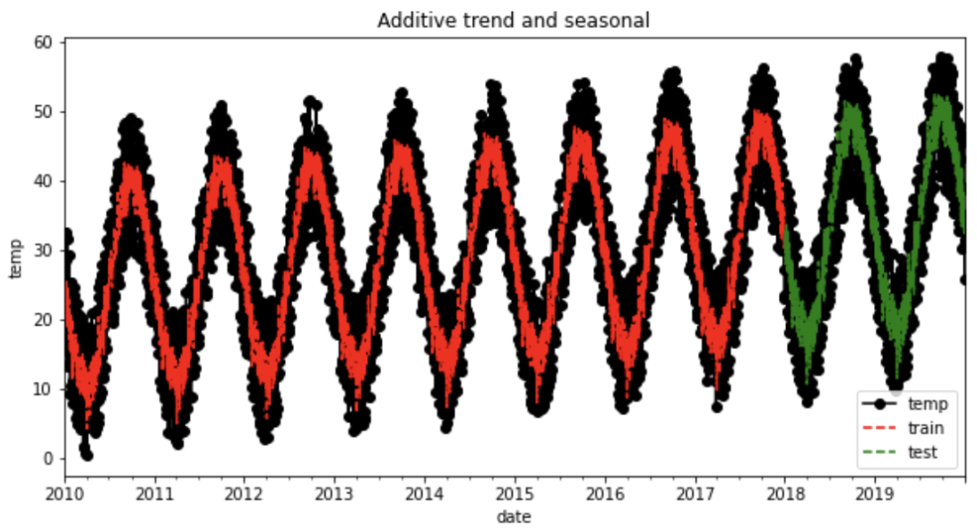
從圖中我們可以觀察到模型是如何捕捉時(shí)間序列的季節(jié)性和趨勢(shì)的，在異常值的預(yù)測(cè)上則存在一些誤差。

總結(jié)

在本文中，我們通過一個(gè)基于溫度數(shù)據(jù)集的實(shí)際示例來介紹趨勢(shì)和季節(jié)性。除了檢查趨勢(shì)和季節(jié)性之外，我們還看到了如何降低它，以及如何創(chuàng)建一個(gè)基本模型，利用這些模式來推斷未來幾天的溫度。

了解主要的時(shí)間序列模式和學(xué)習(xí)如何實(shí)現(xiàn)時(shí)間序列預(yù)測(cè)模型是至關(guān)重要的，因?yàn)樗鼈冇性S多應(yīng)用。


長按或掃描下方二維碼，后臺(tái)回復(fù)：加群，即可申請(qǐng)入群。一定要備注：來源+研究方向+學(xué)校/公司，否則不拉入群中，見諒！
（長按三秒，進(jìn)入后臺(tái)）

推薦閱讀
利用Python做一個(gè)漂亮小姐姐詞云跳舞視頻
30 個(gè)Python代碼實(shí)現(xiàn)的常用功能，精心整理版
神器！三行 Python 代碼輕松提取 PDF 表格數(shù)據(jù)
四款可視化工具，解決99%的可視化大屏需求

基于趨勢(shì)和季節(jié)性的時(shí)間序列預(yù)測(cè)實(shí)戰(zhàn)