欧美中文字幕免费在线观看,黑人大战久久,综合性爱网,亚洲在线资源,操逼网站123,亚洲色图一区二区三区,日皮免费视频成全视频,嫩草网址

點(diǎn)擊上方“小白學(xué)視覺”，選擇加"星標(biāo)"或“置頂”

重磅干貨，第一時(shí)間送達(dá)

深度學(xué)習(xí)是基于人工神經(jīng)網(wǎng)絡(luò)(ANN)的機(jī)器學(xué)習(xí)方法大家庭的一部分。深度學(xué)習(xí)是當(dāng)今普遍存在的一種學(xué)習(xí)方式，它被廣泛應(yīng)用于從圖像分類到語音識(shí)別的各個(gè)領(lǐng)域。在這篇文章中，我將向你展示如何構(gòu)建一個(gè)簡(jiǎn)單的神經(jīng)網(wǎng)絡(luò)，用PyTorch從視網(wǎng)膜光學(xué)相干斷層掃描圖像中檢測(cè)不同的眼部疾病。

數(shù)據(jù)集
OCT 是一種成像技術(shù)，用于捕捉活體患者視網(wǎng)膜的高分辨率橫截面。每年大約要進(jìn)行3000萬次 OCT 掃描，這些圖像的分析和解釋需要大量的時(shí)間。

這個(gè)數(shù)據(jù)集來自 kaggle，它被分成3個(gè)文件夾(train，test，val) ，每個(gè)圖像類別包含子文件夾: 脈絡(luò)膜新血管生成(CNV) ，糖尿病性黃斑水腫(DME) ，早期 AMD (DRUSEN)中出現(xiàn)的多個(gè)視網(wǎng)膜，以及保留中心凹輪廓的正常視網(wǎng)膜，沒有任何視網(wǎng)膜液體/水腫(NORMAL)。

加載和預(yù)處理圖像

首先，我們要加載所有的庫，并指定函數(shù)，我們將用來加載我們的數(shù)據(jù)和模型在 GPU 上。
import torchimport torch.nn as nnimport torch.optim as optimfrom torch.optim import lr_schedulerfrom torch.utils.data import DataLoaderimport torch.nn.functional as F
from PIL import Image
import torchvisionimport torchvision.models as modelsfrom torchvision import datasets, modelsfrom torchvision.utils import make_gridimport torchvision.transforms as tt
import timeimport osfrom itertools import product
from tqdm.notebook import tqdmfrom tqdm import trange
import numpy as npimport pandas as pdimport matplotlib as mplimport matplotlib.pyplot as pltimport matplotlib.image as mpimgimport matplotlib.lines as mlinesfrom matplotlib.ticker import MaxNLocator, FormatStrFormatterplt.style.use(['seaborn-dark'])mpl.rcParams.update({"axes.grid" : True,                      "grid.color": "grey",                     'grid.linestyle':":",})
from sklearn.metrics import accuracy_score, f1_score, precision_score, recall_score, classification_report, ConfusionMatrixDisplay, confusion_matrix
def to_device(data, device):    """Move tensor(s) to chosen device"""    if isinstance(data, (list,tuple)):        return [to_device(x, device) for x in data]    #print(f"Moved to {device}")    return data.to(device, non_blocking=True)
#Pick GPU if available, else CPUif torch.cuda.is_available():    device = torch.device('cuda')else:    device = torch.device('cpu')print(device)cuda
然后我們將解析 train 文件夾中的所有圖像，以創(chuàng)建包含訓(xùn)練圖像的每個(gè)通道的平均值和標(biāo)準(zhǔn)差的兩個(gè)矢量。我們要利用這些數(shù)據(jù)對(duì)圖像進(jìn)行normalize操作。

def get_stats_channels(path="./", batch_size=50):    """    Create two tuples with mean and std for each RGB channel of the dataset    """    data = datasets.ImageFolder(path, tt.Compose([tt.CenterCrop(490),                                                  tt.ToTensor()]))    loader = DataLoader(data, batch_size, num_workers=4, pin_memory=True)
    nimages = 0    mean = 0.    std = 0.    for batch, _ in tqdm(loader):        # Rearrange batch to be the shape of [B, C, W * H]        batch = batch.view(batch.size(0), batch.size(1), -1)        # Update total number of images        nimages += batch.size(0)        # Compute mean and std here        mean += batch.mean(2).sum(0)         std += batch.std(2).sum(0)

    mean /= nimages    std /= nimages
    return mean, std#normalization_stats = get_stats_channels(data_dir+"/"+"train")normalization_stats = (0.1899, 0.1899, 0.1899), (0.1912, 0.1912, 0.1912)#normalization_stats = (0.485, 0, 0), (0.229, 1, 1)現(xiàn)在我們使用 pytorch 加載數(shù)據(jù)。每幅圖像都是中心像素，大小為490x490像素(為了在每幅圖像之間保持統(tǒng)一大小) ，然后轉(zhuǎn)換為張量，再進(jìn)行規(guī)范化。

data_transforms = {    'Train': tt.Compose([tt.CenterCrop(490),                         tt.ToTensor(), tt.Normalize(*normalization_stats)]),    'Valid': tt.Compose([tt.CenterCrop(490),                         tt.ToTensor(), tt.Normalize(*normalization_stats)]),    'Test': tt.Compose([tt.CenterCrop(490),                        tt.ToTensor(), tt.Normalize(*normalization_stats)])}
train_data = datasets.ImageFolder(data_dir+"/"+"train/",                                   transform=data_transforms["Train"])valid_data = datasets.ImageFolder(data_dir+"/"+"val/",                                   transform=data_transforms["Valid"])test_data = datasets.ImageFolder(data_dir+"/"+"test/",                                 transform=data_transforms["Test"])可視化數(shù)據(jù)

現(xiàn)在我們已經(jīng)加載并預(yù)處理了數(shù)據(jù)，我們可以進(jìn)行一些數(shù)據(jù)探索。
CNV = Image.open('../input/kermany2018/OCT2017 /train/CNV/CNV-1016042-1.jpeg')DME = Image.open('../input/kermany2018/OCT2017 /train/DME/DME-1072015-1.jpeg')DRUSEN = Image.open('../input/kermany2018/OCT2017 /train/DRUSEN/DRUSEN-1001666-1.jpeg')NORMAL = Image.open('../input/kermany2018/OCT2017 /train/NORMAL/NORMAL-1001666-1.jpeg')
fig, (ax1, ax2) = plt.subplots(nrows=2, ncols=4, figsize=(10,10))ax1[0].imshow(CNV)ax1[0].set(title="CNV")ax1[0].axis('off')
ax1[1].imshow(DME)ax1[1].set(title="DME")ax1[1].axis('off')
CNVtransform = data_transforms["Train"](CNV.convert('RGB')).permute(1, 2, 0)ax1[2].imshow(CNVtransform)ax1[2].set(title="DME transformed")ax1[2].axis('off')
DMEtransform = data_transforms["Train"](DME.convert('RGB')).permute(1, 2, 0)ax1[3].imshow(DMEtransform)ax1[3].set(title="DME transformed")ax1[3].axis('off')
ax2[0].imshow(DRUSEN)ax2[0].set(title="DRUSEN")ax2[0].axis('off')
ax2[1].imshow(NORMAL)ax2[1].set(title="NORMAL")ax2[1].axis('off')
DRUSENtransform = data_transforms["Train"](DRUSEN.convert('RGB')).permute(1, 2, 0)ax2[2].imshow(DRUSENtransform)ax2[2].set(title="DRUSEN transformed")ax2[2].axis('off')
NORMALtransform = data_transforms["Train"](NORMAL.convert('RGB')).permute(1, 2, 0)ax2[3].imshow(NORMALtransform)ax2[3].set(title="NORMAL transformed")ax2[3].axis('off')
plt.tight_layout()plt.show()
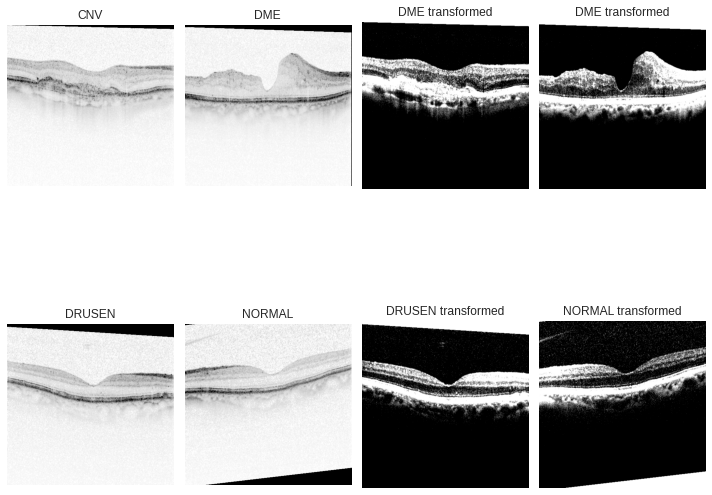
在左邊我們可以看到原始圖像，在右邊我們看到經(jīng)過預(yù)處理的圖像。標(biāo)準(zhǔn)化將所有通道的平均值都集中在零點(diǎn)附近，這種操作有助于網(wǎng)絡(luò)更快地學(xué)習(xí)，因?yàn)樘荻葘?duì)每個(gè)通道的作用是一致的，并有助于在圖像中產(chǎn)生有意義的特征。
fig, (ax1, ax2, ax3) = plt.subplots(nrows=3, ncols=1,                                    figsize=(5,8), sharex=True)train_labels.plot(ax=ax1, kind="bar")ax1.set(title="Train label")
valid_labels.plot(ax=ax2, kind="bar")ax2.set(title="Validation labels")
test_labels.plot(ax=ax3, kind="bar")ax3.set(title="Test labels")
plt.show()

我們繪制訓(xùn)練集標(biāo)簽、驗(yàn)證集標(biāo)簽以及測(cè)試集標(biāo)簽的分布圖便于檢查標(biāo)簽不平衡。我們可以看到，驗(yàn)證集和測(cè)試集中的標(biāo)簽分布是均勻的，而訓(xùn)練集中的標(biāo)簽分布是不平衡的。有不同的方法來處理不平衡的數(shù)據(jù)集，這里我們嘗試了抽樣處理。

加載數(shù)據(jù)
class DeviceDataLoader():    """Wrap a dataloader to move data to a device"""    def __init__(self, dl, device):        self.dl = dl        self.device = device            def __iter__(self):        """Yield a batch of data after moving it to device"""        for b in self.dl:             yield to_device(b, self.device)
    def __len__(self):        """Number of batches"""        return len(self.dl)
batch_size = 30
train_dl = DataLoader(train_data, batch_size=batch_size,                       sampler=ImbalancedDatasetSampler(train_data, num_samples=4000),                       pin_memory=True, num_workers=4)valid_dl =DataLoader(valid_data, batch_size=batch_size,                      shuffle=True, pin_memory=True, num_workers=4)test_dl = DataLoader(test_data, batch_size=batch_size, pin_memory=True, num_workers=4)
train_dl = DeviceDataLoader(train_dl, device)valid_dl = DeviceDataLoader(valid_dl, device)test_dl = DeviceDataLoader(test_dl, device)這里我們使用自定義加載器在 GPU 上加載數(shù)據(jù)。由于 GPU 的內(nèi)存不足以容納數(shù)以千計(jì)的圖像，因此需要批量大小將數(shù)據(jù)以較小的批量輸入模型。訓(xùn)練數(shù)據(jù)集并不是整體加載的，我們使用了一個(gè)自定義的采樣器來對(duì)數(shù)據(jù)進(jìn)行子采樣(為了使每個(gè)標(biāo)簽的分布更加均勻) ，并將訓(xùn)練數(shù)據(jù)總數(shù)減少到4000個(gè)圖像，以加快計(jì)算時(shí)間的速度。

模型
#================================================================================class TransferResnet(nn.Module):    """Feedfoward neural network with 1 hidden layer"""    def __init__(self, classes=4):        super().__init__()        # Use a pretrained model        self.network = models.resnet34(pretrained=True)                #self.network.avgpool = AdaptiveConcatPool2d()        # Replace last layer        num_ftrs = self.network.fc.in_features        self.network.fc = nn.Sequential(nn.Linear(num_ftrs, 128),                                         nn.ReLU(),                                          nn.Dropout(0.50),                                                                                 nn.Linear(128,classes))        def forward(self, xb):        out = self.network(xb)        return out
    def feed_to_network(self, batch):        images, labels = batch         out = self(images)          loss = F.cross_entropy(out, labels)        #Don't pass the softmax to the cross entropy        out = F.softmax(out, dim=1)

        return loss, out
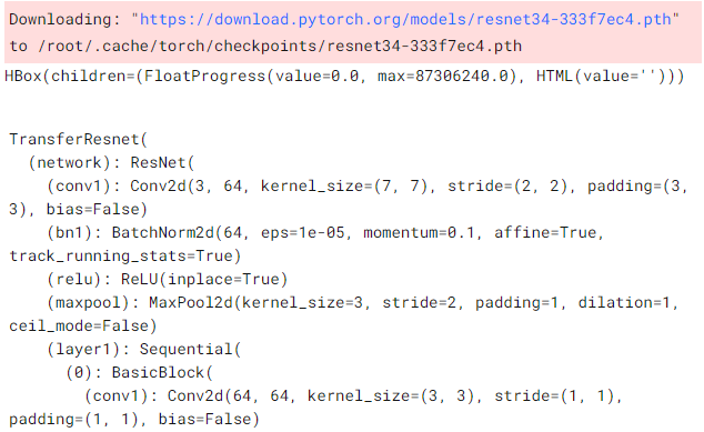
model = TransferResnet()model = to_device(model, device)model
部分結(jié)果

最后我們創(chuàng)建了我們的模型，給出了我們相對(duì)較小的樣本量(并且為了加快訓(xùn)練時(shí)間) ，我們使用了遷移學(xué)習(xí)和 ResNet 的預(yù)訓(xùn)練模型，并刪除了最終的全連接層，并添加了兩個(gè)線性層和一個(gè) ReLu 激活函數(shù)。因?yàn)槲覀冋谧鲆粋€(gè)分類任務(wù)，我們的損失函數(shù)將是交叉熵?fù)p失。

訓(xùn)練模型
def get_scores(labels, prediction, loss=None):    "Return classification scores"    accuracy = accuracy_score(labels, prediction)     f1 = f1_score(labels, prediction,                   average='weighted', zero_division=0)    precision = precision_score(labels, prediction,                                 average='weighted', zero_division=0)    recall = recall_score(labels, prediction,                           average='weighted', zero_division=0)    if loss:        return [accuracy, f1, precision, recall, loss]    else:         return [accuracy, f1, precision, recall]
def get_predictions(model, loader):    """This function takes a model and a data loader,     returns the list of losses, the predictions and the labels"""
    model.eval()
    with torch.no_grad():                losses = []        predictions = []        labels = []                for batch in loader:            loss, out = model.feed_to_network(batch)                        predictions += torch.argmax(out, dim=1).tolist()            labels += batch[1].tolist()            losses.append(loss.item())                    return labels, predictions, sum(losses)/len(losses)
def new_fit(model, train_loader, val_loader,             optimizer=torch.optim.Adam, lr=1e-2, epochs =10):    def get_lr(optimizer):        for param_group in optimizer.param_groups:            return param_group['lr']
    train_metrics_df = pd.DataFrame(columns=['accuracy', 'f1', 'precision',                                              'recall', 'loss'])    valid_metrics_df = pd.DataFrame(columns=['accuracy', 'f1', 'precision',                                              'recall', 'loss'])
    optimizer = optimizer([{"params": model.network.fc.parameters(), "lr": lr},                           {"params": model.network.layer4.parameters(), "lr": lr/2.5},                           {"params": model.network.layer3.parameters(), "lr": lr/5},                           {"params": model.network.layer2.parameters(), "lr": lr/10},                           {"params": model.network.layer1.parameters(), "lr": lr/100},], lr, weight_decay=1e-5)
    sched = torch.optim.lr_scheduler.ReduceLROnPlateau(optimizer, patience=3)
    lr_list = []    for epoch in range(epochs):                model.train()                lr_list.append(get_lr(optimizer))
                train_label = []        train_prediction = []        train_losses = []
        for batch in tqdm(train_loader):            optimizer.zero_grad()            loss, out = model.feed_to_network(batch)            loss.backward()            optimizer.step()                                    #momentum_list.append(get_parameter(optimizer, parameter="momentum"))            #lr_list.append(get_parameter(optimizer, parameter="lr"))                                    #Extract labels, predictions and loss of the training set            train_prediction += torch.argmax(out, dim=1).tolist()            train_label += batch[1].tolist()            train_losses.append(loss.item())                #Evaluation phase        val_labels, val_predictions, val_loss = get_predictions(model, val_loader)                train_metrics_df.loc[epoch] = get_scores(train_label,train_prediction,                                                 loss=sum(train_losses)/len(train_losses))        valid_metrics_df.loc[epoch] = get_scores(val_labels, val_predictions,                                                  loss=val_loss)                        print_epoch_trainLoss = train_metrics_df.iloc[epoch]["loss"]        print_epoch_validLoss = valid_metrics_df.iloc[epoch]["loss"]        print_epoch_validAccu = valid_metrics_df.iloc[epoch]["accuracy"]        print_epoch_trainAccu = train_metrics_df.iloc[epoch]["accuracy"]                sched.step(print_epoch_trainLoss)
                print(f"\t\tEpoch {epoch+1}\t\n"              f"Train loss:{train_losses[-1]:.4f}\tValid loss:{print_epoch_validLoss:.4f}\n"              f"Train acc :{print_epoch_trainAccu*100:.2f}\tValid acc :{print_epoch_validAccu*100:.2f}")            return train_metrics_df, valid_metrics_df, lr_list一個(gè)經(jīng)過訓(xùn)練的模型是有用的，因?yàn)樗膶右呀?jīng)被訓(xùn)練來提取特征(比如特定的形狀或線條，等等)。因此，在訓(xùn)練過程中，網(wǎng)絡(luò)卷積部分的權(quán)重和偏差不會(huì)發(fā)生很大變化。另一方面，我們創(chuàng)建的全連接層是用隨機(jī)權(quán)重初始化的。解決這個(gè)問題的一個(gè)方法是凍結(jié)網(wǎng)絡(luò)中所有預(yù)先訓(xùn)練的部分，只訓(xùn)練最后的全連接層，然后解凍所有的網(wǎng)絡(luò)，以較低的學(xué)習(xí)率訓(xùn)練它。我們采用了另一種技術(shù)：我們對(duì)網(wǎng)絡(luò)的每個(gè)部分使用不同的學(xué)習(xí)速度。更深的網(wǎng)絡(luò)層使用更低的學(xué)習(xí)率。通過這種方法，我們訓(xùn)練了分類器，并對(duì)預(yù)訓(xùn)練的網(wǎng)絡(luò)進(jìn)行了微調(diào)，而無需對(duì)其進(jìn)行兩次訓(xùn)練。

作為一個(gè)例子，我們使用 Adam 優(yōu)化器對(duì)這個(gè)網(wǎng)絡(luò)進(jìn)行了15個(gè) epoch 的訓(xùn)練，學(xué)習(xí)率為0.004，并使用了一個(gè)學(xué)習(xí)率調(diào)度器。

計(jì)劃學(xué)習(xí)率是非常有用的，因?yàn)楦邔W(xué)習(xí)速率有助于網(wǎng)絡(luò)學(xué)習(xí)更快，但他們有可能錯(cuò)過最小的損失函數(shù)。另一方面，低學(xué)習(xí)率可能太慢了。
我們使用了一個(gè)調(diào)度器，降低了學(xué)習(xí)率一旦它停止，以減少損失函數(shù)。我們繪制每個(gè) epoch 的損失函數(shù)、學(xué)習(xí)速度和不同的分類指標(biāo)：

colors = plt.rcParams['axes.prop_cycle'].by_key()['color']
fig = plt.figure(constrained_layout=True, figsize=(8,5))gs = fig.add_gridspec(nrows=4, ncols=2)
fig_ax1 = fig.add_subplot(gs[0, :])fig_ax1.plot(train_metrics_df["loss"], label="train")fig_ax1.plot(valid_metrics_df["loss"])fig_ax1.xaxis.set_major_locator(MaxNLocator(integer=True))fig_ax1.set(title='Loss')fig_ax1.set_ylim(bottom=0)
fig_ax2 = fig.add_subplot(gs[1, 0])fig_ax2.plot(train_metrics_df["accuracy"], label="train")fig_ax2.plot(valid_metrics_df["accuracy"], label="validation")fig_ax2.xaxis.set_major_locator(MaxNLocator(integer=True))fig_ax2.set(title="Accuracy", ylim=(0,1))
fig_ax3 = fig.add_subplot(gs[1, 1])fig_ax3.plot(train_metrics_df["f1"], label="train")fig_ax3.plot(valid_metrics_df["f1"], label="validation")fig_ax3.xaxis.set_major_locator(MaxNLocator(integer=True))fig_ax3.set(title="F1", ylim=(0,1))
fig_ax4 = fig.add_subplot(gs[2, 0])fig_ax4.plot(train_metrics_df["precision"], label="train")fig_ax4.plot(valid_metrics_df["precision"], label="validation")fig_ax4.xaxis.set_major_locator(MaxNLocator(integer=True))fig_ax4.set(title="Rrecision", ylim=(0,1))
fig_ax5 = fig.add_subplot(gs[2, 1])fig_ax5.plot(train_metrics_df["recall"], label="train")fig_ax5.plot(valid_metrics_df["recall"], label="validation")fig_ax5.xaxis.set_major_locator(MaxNLocator(integer=True))fig_ax5.set(title="Recall", ylim=(0,1))
fig_ax6 = fig.add_subplot(gs[3, :])fig_ax6.plot(lr_list, label="learning rate", color=colors[2])fig_ax6.xaxis.set_major_locator(MaxNLocator(integer=True))fig_ax6.set(title='Learning Rate')fig_ax6.set_ylim(bottom=0)

dummytrain = mlines.Line2D([], [], color=colors[0], label='Train set')dummyvalid = mlines.Line2D([], [], color=colors[1], label='Validation set')dummyrate = mlines.Line2D([], [], color=colors[2], label='Learning Rate')

fig.legend([dummytrain, dummyvalid,dummyrate],            ["Training set", "Validation set", "Learning Rate"],           bbox_to_anchor=(1.05, 1), loc='upper left', borderaxespad=0.)
plt.show()
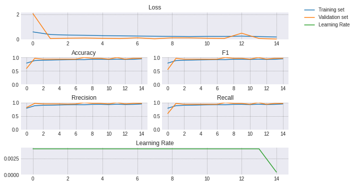
所有的指標(biāo)在短短幾個(gè)時(shí)期內(nèi)就達(dá)到了0.9，在訓(xùn)練結(jié)束時(shí)驗(yàn)證的準(zhǔn)確率達(dá)到了93.75% ，對(duì)于一個(gè)簡(jiǎn)單的網(wǎng)絡(luò)來說，這已經(jīng)不錯(cuò)了！

測(cè)試模型

最后，我們使用測(cè)試集來測(cè)試模型。首先讓我們看看相關(guān)矩陣：
cm = confusion_matrix(test_labels, test_predictions, normalize="pred")

fig, ax = plt.subplots(figsize=(8,6))im = ax.imshow(cm, cmap="viridis")fig.colorbar(im)
ax.set(xticks=np.arange(len(labels)),        yticks=np.arange(len(labels)),        xticklabels=labels,        yticklabels=labels,       ylabel="True labels",       xlabel="Predicted labels")

# Rotate the tick labels and set their alignment.plt.setp(ax.get_xticklabels(), rotation=45, ha="right",         rotation_mode="anchor")
# Loop over data dimensions and create text annotations.cmap_min, cmap_max = im.cmap(0), im.cmap(256)for i,j in product(range(len(labels)),range(len(labels))):    color = cmap_max if cm[i,j] < cm.max()/4 else cmap_min
    text = ax.text(j, i, round(cm[i, j],2),ha="center", va="center", color=color)

ax.set_title("Confusion matrix of the test set")fig.tight_layout()plt.show()
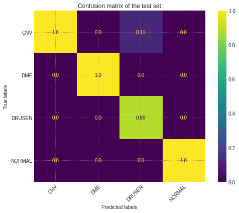
這幾乎是完美的！該模型能夠正確地對(duì)幾乎所有的標(biāo)簽進(jìn)行分類，其中11% 的 DRUSEN 圖像混淆為 CNV。現(xiàn)在讓我們來看看測(cè)試集的度量：

labels = ['CNV', 'DME', 'DRUSEN', 'NORMAL']test_labels, test_predictions, _ = get_predictions(model, valid_dl)print(classification_report(test_labels, test_predictions,                             zero_division = 0, target_names=labels))
最后，測(cè)試集上的所有度量值都是0.97，甚至高于驗(yàn)證集！

這個(gè)網(wǎng)絡(luò)表現(xiàn)很好，但是它還可以改進(jìn)：

更多的 epoch ：由于時(shí)間限制，我們只訓(xùn)練了15個(gè) epoch，使用更多的 epoch 可以極大地提高準(zhǔn)確性；
早期停止：使用更多的時(shí)期，我們可以避免數(shù)據(jù)過擬合的風(fēng)險(xiǎn)和增加泛化誤差，早期停止訓(xùn)練，避免為了過度擬合測(cè)試集引起的驗(yàn)證集的loss爆炸；
改變參數(shù)：學(xué)習(xí)速度，權(quán)重衰減等。所有的參數(shù)均可以調(diào)整，以提高準(zhǔn)確性；
使用數(shù)據(jù)增強(qiáng)：增加隨機(jī)旋轉(zhuǎn)、裁剪等等可以幫助模型更好地泛化。

使用 PyTorch 檢測(cè)眼部疾病