PyTorch 源碼解讀之 torch.autograd
AI編輯:我是小將
本文作者:?OpenMMLab @000255
https://zhuanlan.zhihu.com/p/321449610
本文已由原作者授權(quán)
前言
本篇筆記以介紹 pytorch 中的 autograd 模塊功能為主,主要涉及 torch/autograd 下代碼,不涉及底層的 C++ 實(shí)現(xiàn)。本文涉及的源碼以 PyTorch 1.7 為準(zhǔn)。
torch.autograd.function (函數(shù)的反向傳播)
torch.autograd.functional (計(jì)算圖的反向傳播)
torch.autograd.gradcheck (數(shù)值梯度檢查)
torch.autograd.anomaly_mode (在自動(dòng)求導(dǎo)時(shí)檢測(cè)錯(cuò)誤產(chǎn)生路徑)
torch.autograd.grad_mode (設(shè)置是否需要梯度)
model.eval() 與 torch.no_grad()
torch.autograd.profiler (提供 function 級(jí)別的統(tǒng)計(jì)信息)
torch.autograd.function?(函數(shù)的反向傳播)
我們?cè)跇?gòu)建網(wǎng)絡(luò)的時(shí)候,通常使用 pytorch 所提供的nn.Module?(例如nn.Conv2d,?nn.ReLU等)作為基本單元。而這些 Module 通常是包裹 autograd function,以其作為真正實(shí)現(xiàn)的部分。例如nn.ReLU?實(shí)際使用torch.nn.functional.relu(F.relu):
from torch.nn import functional as F

class ReLU(Module):
    __constants__ = ['inplace']
    inplace: bool

    def __init__(self, inplace: bool = False):
        super(ReLU, self).__init__()
        self.inplace = inplace

    def forward(self, input: Tensor) -> Tensor:
return F.relu(input, inplace=self.inplace)這里的F.relu類(lèi)型為function,若再剝開(kāi)一層,其實(shí)際包裹的函數(shù)類(lèi)型為builtin_function_or_method,這也是真正完成運(yùn)算的部分。這些部分通常使用 C++ 實(shí)現(xiàn)(如ATen)。至此我們知道,一個(gè)模型的運(yùn)算部分由 autograd functions 組成,這些 autograd functions 內(nèi)部定義了 forward,backward 用以描述前向和梯度反傳的過(guò)程,組合后可以實(shí)現(xiàn)整個(gè)模型的前向和梯度反傳。以torch.autograd.function中所定義的Function類(lèi)為基類(lèi),我們可以實(shí)現(xiàn)自定義的autograd function,所實(shí)現(xiàn)的 function 需包含forward及backward兩個(gè)方法。以下以Exp和GradCoeff兩個(gè)自定義 autograd function 為例進(jìn)行講解:
class Exp(Function):                    # 此層計(jì)算e^x

    @staticmethod
    def forward(ctx, i):                # 模型前向
        result = i.exp()
        ctx.save_for_backward(result)   # 保存所需內(nèi)容,以備backward時(shí)使用,所需的結(jié)果會(huì)被保存在saved_tensors元組中;此處僅能保存tensor類(lèi)型變量,若其余類(lèi)型變量(Int等),可直接賦予ctx作為成員變量,也可以達(dá)到保存效果
        return result

    @staticmethod
    def backward(ctx, grad_output):     # 模型梯度反傳
        result, = ctx.saved_tensors     # 取出forward中保存的result
        return grad_output * result     # 計(jì)算梯度并返回

# 嘗試使用
x = torch.tensor([1.], requires_grad=True)  # 需要設(shè)置tensor的requires_grad屬性為T(mén)rue,才會(huì)進(jìn)行梯度反傳
ret = Exp.apply(x)                          # 使用apply方法調(diào)用自定義autograd function
print(ret)                                  # tensor([2.7183], grad_fn=)
ret.backward()                              # 反傳梯度
print(x.grad)                               # tensor([2.7183])
Exp 函數(shù)的前向很簡(jiǎn)單,直接調(diào)用 tensor 的成員方法exp即可。反向時(shí),我們知道? ?, 因此我們直接使用?
 ?乘以
?乘以grad_output即得梯度。我們發(fā)現(xiàn),我們自定義的函數(shù)Exp正確地進(jìn)行了前向與反向。同時(shí)我們還注意到,前向后所得的結(jié)果包含了grad_fn屬性,這一屬性指向用于計(jì)算其梯度的函數(shù)(即Exp的backward函數(shù))。關(guān)于這點(diǎn),在接下來(lái)的部分會(huì)有更詳細(xì)的說(shuō)明。接下來(lái)我們看另一個(gè)函數(shù)GradCoeff,其功能是反傳梯度時(shí)乘以一個(gè)自定義系數(shù)。
class GradCoeff(Function):

    @staticmethod
    def forward(ctx, x, coeff):                 # 模型前向
        ctx.coeff = coeff                       # 將coeff存為ctx的成員變量
        return x.view_as(x)

    @staticmethod
    def backward(ctx, grad_output):             # 模型梯度反傳
        return ctx.coeff * grad_output, None    # backward的輸出個(gè)數(shù),應(yīng)與forward的輸入個(gè)數(shù)相同,此處coeff不需要梯度,因此返回None

# 嘗試使用
x = torch.tensor([2.], requires_grad=True)
ret = GradCoeff.apply(x, -0.1)                  # 前向需要同時(shí)提供x及coeff,設(shè)置coeff為-0.1
ret = ret ** 2
print(ret)                                      # tensor([4.], grad_fn=)
ret.backward()
print(x.grad) # tensor([-0.4000]),梯度已乘以相應(yīng)系數(shù)torch.autograd.functional?(計(jì)算圖的反向傳播)
在此前一節(jié),我們描述了單個(gè)函數(shù)的反向傳播,以及如何編寫(xiě)定制的 autograd function。在這一節(jié)中,我們簡(jiǎn)單介紹 pytorch 中所提供的計(jì)算圖反向傳播的接口。
在訓(xùn)練過(guò)程中,我們通常利用 prediction 和 groundtruth label 來(lái)計(jì)算 loss(loss 的類(lèi)型為T(mén)ensor),隨后調(diào)用loss.backward()進(jìn)行梯度反傳。而 Tensor 類(lèi)的backward方法,實(shí)際調(diào)用的就是torch.autograd.backward這一接口。這一 python 接口實(shí)現(xiàn)了計(jì)算圖級(jí)的反向傳播。
class Tensor(torch._C._TensorBase)

    def backward(self, gradient=None, retain_graph=None, create_graph=False):
        relevant_args = (self,)
        ...
        torch.autograd.backward(self, gradient, retain_graph, create_graph)
        # gradient: 形狀與tensor一致,可以理解為鏈?zhǔn)角髮?dǎo)的中間結(jié)果,若tensor標(biāo)量,可以省略(默認(rèn)為1)
        # retain_graph: 多次反向傳播時(shí)梯度累加。反向傳播的中間緩存會(huì)被清空,為進(jìn)行多次反向傳播需指定retain_graph=True來(lái)保存這些緩存。
        # create_graph: 為反向傳播的過(guò)程同樣建立計(jì)算圖,可用于計(jì)算二階導(dǎo)
在 pytorch 實(shí)現(xiàn)中,autograd 會(huì)隨著用戶(hù)的操作,記錄生成當(dāng)前 variable 的所有操作,并建立一個(gè)有向無(wú)環(huán)圖 (DAG)。圖中記錄了操作Function,每一個(gè)變量在圖中的位置可通過(guò)其grad_fn屬性在圖中的位置推測(cè)得到。在反向傳播過(guò)程中,autograd 沿著這個(gè)圖從當(dāng)前變量(根節(jié)點(diǎn)?F)溯源,可以利用鏈?zhǔn)角髮?dǎo)法則計(jì)算所有葉子節(jié)點(diǎn)的梯度。每一個(gè)前向傳播操作的函數(shù)都有與之對(duì)應(yīng)的反向傳播函數(shù)用來(lái)計(jì)算輸入的各個(gè) variable 的梯度,這些函數(shù)的函數(shù)名通常以Backward結(jié)尾。我們構(gòu)建一個(gè)簡(jiǎn)化的計(jì)算圖,并以此為例進(jìn)行簡(jiǎn)單介紹。
A = torch.tensor(2., requires_grad=True)
B = torch.tensor(.5, requires_grad=True)
E = torch.tensor(1., requires_grad=True)
C = A * B
D = C.exp()
F = D + E
print(F)        # tensor(3.7183, grad_fn=) 打印計(jì)算結(jié)果,可以看到F的grad_fn指向AddBackward,即產(chǎn)生F的運(yùn)算
print([x.is_leaf for x in [A, B, C, D, E, F]])  # [True, True, False, False, True, False] 打印是否為葉節(jié)點(diǎn),由用戶(hù)創(chuàng)建,且requires_grad設(shè)為T(mén)rue的節(jié)點(diǎn)為葉節(jié)點(diǎn)
print([x.grad_fn for x in [F, D, C, A]])    # [, , , None]  每個(gè)變量的grad_fn指向產(chǎn)生其算子的backward function,葉節(jié)點(diǎn)的grad_fn為空
print(F.grad_fn.next_functions) # ((, 0), (, 0)) 由于F = D + E, 因此F.grad_fn.next_functions也存在兩項(xiàng),分別對(duì)應(yīng)于D, E兩個(gè)變量,每個(gè)元組中的第一項(xiàng)對(duì)應(yīng)于相應(yīng)變量的grad_fn,第二項(xiàng)指示相應(yīng)變量是產(chǎn)生其op的第幾個(gè)輸出。E作為葉節(jié)點(diǎn),其上沒(méi)有g(shù)rad_fn,但有梯度累積函數(shù),即AccumulateGrad(由于反傳時(shí)多出可能產(chǎn)生梯度,需要進(jìn)行累加)
F.backward(retain_graph=True)   # 進(jìn)行梯度反傳
print(A.grad, B.grad, E.grad)   # tensor(1.3591) tensor(5.4366) tensor(1.) 算得每個(gè)變量梯度,與求導(dǎo)得到的相符
print(C.grad, D.grad)   # None None 為節(jié)約空間,梯度反傳完成后,中間節(jié)點(diǎn)的梯度并不會(huì)保留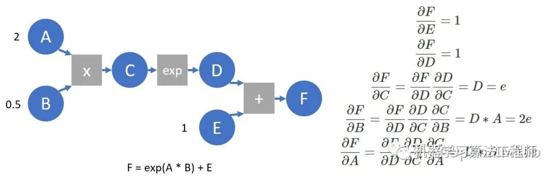
我們?cè)賮?lái)看下面的計(jì)算圖,并在這個(gè)計(jì)算圖上模擬 autograd 所做的工作:
A = torch.tensor([3.], requires_grad=True)
B = torch.tensor([2.], requires_grad=True)
C = A ** 2
D = B ** 2
E = C * D
F = D + E

F.manual_grad = torch.tensor(1)                             # 我們用manual_grad表示,在已知計(jì)算圖結(jié)構(gòu)的情況下,我們模擬autograd過(guò)程手動(dòng)算得的梯度
D.manual_grad, E.manual_grad = F.grad_fn(F.manual_grad)
C.manual_grad, tmp2 = E.grad_fn(E.manual_grad)
D.manual_grad = D.manual_grad + tmp2                        # 這里我們先完成D上的梯度累加,再進(jìn)行反傳
A.manual_grad = C.grad_fn(C.manual_grad)
B.manual_grad = D.grad_fn(D.manual_grad) # (tensor([24.], grad_fn=), tensor([40.], grad_fn=)) 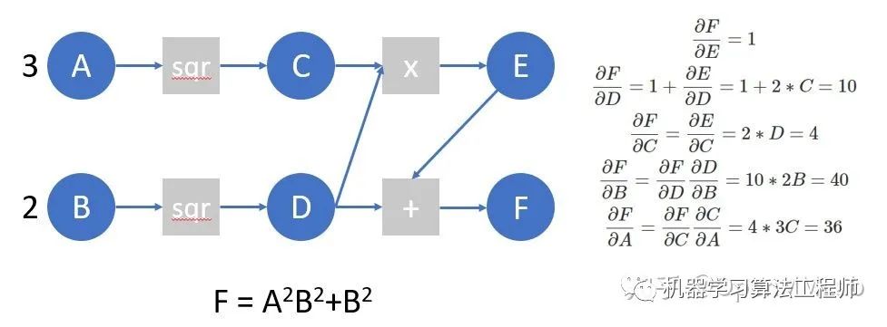
下面,我們編寫(xiě)一個(gè)簡(jiǎn)單的函數(shù),在這個(gè)計(jì)算圖上進(jìn)行autograd,并驗(yàn)證結(jié)果是否正確:
# 這一例子僅可用于每個(gè)op只產(chǎn)生一個(gè)輸出的情況,且效率很低(由于對(duì)于某一節(jié)點(diǎn),每次未等待所有梯度反傳至此節(jié)點(diǎn),就直接將本次反傳回的梯度直接反傳至葉節(jié)點(diǎn))
def autograd(grad_fn, gradient):
    auto_grad = {}
    queue = [[grad_fn, gradient]]
    while queue != []:
        item = queue.pop()
        gradients = item[0](item[1])
        functions = [x[0] for x in item[0].next_functions]
        if type(gradients) is not tuple:
            gradients = (gradients, )
        for grad, func in zip(gradients, functions):
            if type(func).__name__ == 'AccumulateGrad':
                if hasattr(func.variable, 'auto_grad'):
                    func.variable.auto_grad = func.variable.auto_grad + grad
                else:
                    func.variable.auto_grad = grad
            else:
                queue.append([func, grad])

A = torch.tensor([3.], requires_grad=True)
B = torch.tensor([2.], requires_grad=True)
C = A ** 2
D = B ** 2
E = C * D
F = D + E

autograd(F.grad_fn, torch.tensor(1))
print(A.auto_grad, B.auto_grad)         # tensor(24., grad_fn=) tensor(40., grad_fn=)

# 這一autograd同樣可作用于編寫(xiě)的模型,我們將會(huì)看到,它與pytorch自帶的backward產(chǎn)生了同樣的結(jié)果
from torch import nn

class MLP(nn.Module):
    def __init__(self):
        super().__init__()
        self.fc1 = nn.Linear(10, 5)
        self.relu = nn.ReLU()
        self.fc2 = nn.Linear(5, 2)
        self.fc3 = nn.Linear(5, 2)
        self.fc4 = nn.Linear(2, 2)

    def forward(self, x):
        x = self.fc1(x)
        x = self.relu(x)
        x1 = self.fc2(x)
        x2 = self.fc3(x)
        x2 = self.relu(x2)
        x2 = self.fc4(x2)
        return x1 + x2

x = torch.ones([10], requires_grad=True)
mlp = MLP()
mlp_state_dict = mlp.state_dict()

# 自定義autograd
mlp = MLP()
mlp.load_state_dict(mlp_state_dict)
y = mlp(x)
z = torch.sum(y)
autograd(z.grad_fn, torch.tensor(1.))
print(x.auto_grad) # tensor([-0.0121,  0.0055, -0.0756, -0.0747,  0.0134,  0.0867, -0.0546,  0.1121, -0.0934, -0.1046], grad_fn=)

mlp = MLP()
mlp.load_state_dict(mlp_state_dict)
y = mlp(x)
z = torch.sum(y)
z.backward()
print(x.grad) # tensor([-0.0121,  0.0055, -0.0756, -0.0747,  0.0134,  0.0867, -0.0546,  0.1121, -0.0934, -0.1046])
pytorch 使用動(dòng)態(tài)圖,它的計(jì)算圖在每次前向傳播時(shí)都是從頭開(kāi)始構(gòu)建,所以它能夠使用python 控制語(yǔ)句(如 for、if 等)根據(jù)需求創(chuàng)建計(jì)算圖。下面提供一個(gè)例子:
def f(x):
    result = 1
    for ii in x:
        if ii.item()>0: result=ii*result
    return result

x = torch.tensor([0.3071,  1.1043,  1.3605, -0.3471], requires_grad=True)
y = f(x)    # y = x[0]*x[1]*x[2]
y.backward()
print(x.grad)   # tensor([1.5023, 0.4178, 0.3391, 0.0000])

x = torch.tensor([ 1.2817,  1.7840, -1.7033,  0.1302], requires_grad=True)
y = f(x)    # y = x[0]*x[1]*x[3]
y.backward()
print(x.grad) # tensor([0.2323, 0.1669, 0.0000, 2.2866])此前的例子使用的是Tensor.backward()接口(內(nèi)部調(diào)用autograd.backward),下面我們來(lái)介紹autograd提供的jacobian()和hessian()接口,并直接利用其進(jìn)行自動(dòng)微分。這兩個(gè)函數(shù)的輸入為運(yùn)算函數(shù)(接受輸入 tensor,返回輸出 tensor)和輸入 tensor,返回 jacobian 和 hessian 矩陣。對(duì)于jacobian接口,輸入輸出均可以為 n 維張量,對(duì)于hessian接口,輸出必需為一標(biāo)量。jacobian返回的張量 shape 為output_dim x input_dim(若函數(shù)輸出為標(biāo)量,則 output_dim 可省略),hessian返回的張量為input_dim x input_dim。除此之外,這兩個(gè)自動(dòng)微分接口同時(shí)支持運(yùn)算函數(shù)接收和輸出多個(gè) tensor。
from torch.autograd.functional import jacobian, hessian
from torch.nn import Linear, AvgPool2d

fc = Linear(4, 2)
pool = AvgPool2d(kernel_size=2)

def scalar_func(x):
    y = x ** 2
    z = torch.sum(y)
    return z

def vector_func(x):
    y = fc(x)
    return y

def mat_func(x):
    x = x.reshape((1, 1,) + x.shape)
    x = pool(x)
    x = x.reshape(x.shape[2:])
    return x ** 2

vector_input = torch.randn(4, requires_grad=True)
mat_input = torch.randn((4, 4), requires_grad=True)

j = jacobian(scalar_func, vector_input)
assert j.shape == (4, )
assert torch.all(jacobian(scalar_func, vector_input) == 2 * vector_input)
h = hessian(scalar_func, vector_input)
assert h.shape == (4, 4)
assert torch.all(hessian(scalar_func, vector_input) == 2 * torch.eye(4))
j = jacobian(vector_func, vector_input)
assert j.shape == (2, 4)
assert torch.all(j == fc.weight)
j = jacobian(mat_func, mat_input)
assert j.shape == (2, 2, 4, 4)在此前的例子中,我們已經(jīng)介紹了,autograd.backward()為節(jié)約空間,僅會(huì)保存葉節(jié)點(diǎn)的梯度。若我們想得知輸出關(guān)于某一中間結(jié)果的梯度,我們可以選擇使用autograd.grad()接口,或是使用hook機(jī)制:
A = torch.tensor(2., requires_grad=True)
B = torch.tensor(.5, requires_grad=True)
C = A * B
D = C.exp()
torch.autograd.grad(D, (C, A))  # (tensor(2.7183), tensor(1.3591)), 返回的梯度為tuple類(lèi)型, grad接口支持對(duì)多個(gè)變量計(jì)算梯度

def variable_hook(grad):                        # hook注冊(cè)在Tensor上,輸入為反傳至這一tensor的梯度
    print('the gradient of C is:', grad)

A = torch.tensor(2., requires_grad=True)
B = torch.tensor(.5, requires_grad=True)
C = A * B
hook_handle = C.register_hook(variable_hook)    # 在中間變量C上注冊(cè)hook
D = C.exp()
D.backward()                                    # 反傳時(shí)打印:the gradient of C is:tensor(2.7183)
hook_handle.remove() # 如不再需要,可remove掉這一hooktorch.autograd.gradcheck?(數(shù)值梯度檢查)
在編寫(xiě)好自己的 autograd function 后,可以利用gradcheck中提供的gradcheck和gradgradcheck接口,對(duì)數(shù)值算得的梯度和求導(dǎo)算得的梯度進(jìn)行比較,以檢查backward是否編寫(xiě)正確。以函數(shù)? ?為例,數(shù)值法求得?
 ?點(diǎn)的梯度為:?
 ?。在下面的例子中,我們自己實(shí)現(xiàn)了
Sigmoid函數(shù),并利用gradcheck來(lái)檢查backward的編寫(xiě)是否正確。
class Sigmoid(Function):

    @staticmethod
    def forward(ctx, x):
        output = 1 / (1 + torch.exp(-x))
        ctx.save_for_backward(output)
        return output

    @staticmethod
    def backward(ctx, grad_output):
        output,  = ctx.saved_tensors
        grad_x = output * (1 - output) * grad_output
        return grad_x

test_input = torch.randn(4, requires_grad=True)     # tensor([-0.4646, -0.4403,  1.2525, -0.5953], requires_grad=True)
torch.autograd.gradcheck(Sigmoid.apply, (test_input,), eps=1e-3)    # pass
torch.autograd.gradcheck(torch.sigmoid, (test_input,), eps=1e-3)    # pass
torch.autograd.gradcheck(Sigmoid.apply, (test_input,), eps=1e-4)    # fail
torch.autograd.gradcheck(torch.sigmoid, (test_input,), eps=1e-4)    # fail
我們發(fā)現(xiàn):eps 為 1e-3 時(shí),我們編寫(xiě)的 Sigmoid 和 torch 自帶的 builtin Sigmoid 都可以通過(guò)梯度檢查,但 eps 下降至 1e-4 時(shí),兩者反而都無(wú)法通過(guò)。而一般直覺(jué)下,計(jì)算數(shù)值梯度時(shí), eps 越小,求得的值應(yīng)該更接近于真實(shí)的梯度。這里的反常現(xiàn)象,是由于機(jī)器精度帶來(lái)的誤差所致:test_input的類(lèi)型為torch.float32,因此在 eps 過(guò)小的情況下,產(chǎn)生了較大的精度誤差(計(jì)算數(shù)值梯度時(shí),eps 作為被除數(shù)),因而與真實(shí)精度間產(chǎn)生了較大的 gap。將test_input換為float64的 tensor 后,不再出現(xiàn)這一現(xiàn)象。這點(diǎn)同時(shí)提醒我們,在編寫(xiě)backward時(shí),要考慮的數(shù)值計(jì)算的一些性質(zhì),盡可能保留更精確的結(jié)果。
test_input = torch.randn(4, requires_grad=True, dtype=torch.float64)    # tensor([-0.4646, -0.4403,  1.2525, -0.5953], dtype=torch.float64, requires_grad=True)
torch.autograd.gradcheck(Sigmoid.apply, (test_input,), eps=1e-4)    # pass
torch.autograd.gradcheck(torch.sigmoid, (test_input,), eps=1e-4)    # pass

torch.autograd.gradcheck(Sigmoid.apply, (test_input,), eps=1e-6)    # pass
torch.autograd.gradcheck(torch.sigmoid, (test_input,), eps=1e-6) # passtorch.autograd.anomaly_mode?(在自動(dòng)求導(dǎo)時(shí)檢測(cè)錯(cuò)誤產(chǎn)生路徑)
可用于在自動(dòng)求導(dǎo)時(shí)檢測(cè)錯(cuò)誤產(chǎn)生路徑,借助with autograd.detect_anomaly():?或是?torch.autograd.set_detect_anomaly(True)來(lái)啟用:
>>> import torch
>>> from torch import autograd
>>>
>>> class MyFunc(autograd.Function):
...
...     @staticmethod
...     def forward(ctx, inp):
...         return inp.clone()
...
...     @staticmethod
...     def backward(ctx, gO):
...         # Error during the backward pass
...         raise RuntimeError("Some error in backward")
...         return gO.clone()
>>>
>>> def run_fn(a):
...     out = MyFunc.apply(a)
...     return out.sum()
>>>
>>> inp = torch.rand(10, 10, requires_grad=True)
>>> out = run_fn(inp)
>>> out.backward()
    Traceback (most recent call last):
      Some Error Log
    RuntimeError: Some error in backward
>>> with autograd.detect_anomaly():
...     inp = torch.rand(10, 10, requires_grad=True)
...     out = run_fn(inp)
...     out.backward()
    Traceback of forward call that caused the error:            # 檢測(cè)到錯(cuò)誤發(fā)生的Trace
      File "tmp.py", line 53, in <module>
        out = run_fn(inp)
      File "tmp.py", line 44, in run_fn
        out = MyFunc.apply(a)
    Traceback (most recent call last):
      Some Error Log
RuntimeError: Some error in backwardtorch.autograd.grad_mode?(設(shè)置是否需要梯度)
我們?cè)?inference 的過(guò)程中,不希望 autograd 對(duì) tensor 求導(dǎo),因?yàn)榍髮?dǎo)需要緩存許多中間結(jié)構(gòu),增加額外的內(nèi)存/顯存開(kāi)銷(xiāo)。在 inference 時(shí),關(guān)閉自動(dòng)求導(dǎo)可實(shí)現(xiàn)一定程度的速度提升,并節(jié)省大量?jī)?nèi)存及顯存(被節(jié)省的不僅限于原先用于梯度存儲(chǔ)的部分)。我們可以利用grad_mode中的troch.no_grad()來(lái)關(guān)閉自動(dòng)求導(dǎo):
from torchvision.models import resnet50
import torch

net = resnet50().cuda(0)
num = 128
inp = torch.ones([num, 3, 224, 224]).cuda(0)
net(inp)                                        # 若不開(kāi)torch.no_grad(),batch_size為128時(shí)就會(huì)OOM (在1080 Ti上)

net = resnet50().cuda(1)
num = 512
inp = torch.ones([num, 3, 224, 224]).cuda(1)
with torch.no_grad():                           # 打開(kāi)torch.no_grad()后,batch_size為512時(shí)依然能跑inference (節(jié)約超過(guò)4倍顯存)
net(inp)model.eval()與torch.no_grad()
這兩項(xiàng)實(shí)際無(wú)關(guān),在 inference 的過(guò)程中需要都打開(kāi):model.eval()令 model 中的BatchNorm,?Dropout等 module 采用 eval mode,保證 inference 結(jié)果的正確性,但不起到節(jié)省顯存的作用;torch.no_grad()聲明不計(jì)算梯度,節(jié)省大量?jī)?nèi)存和顯存。
torch.autograd.profiler?(提供function級(jí)別的統(tǒng)計(jì)信息)
import torch
from torchvision.models import resnet18

x = torch.randn((1, 3, 224, 224), requires_grad=True)
model = resnet18()
with torch.autograd.profiler.profile() as prof:
    for _ in range(100):
        y = model(x)
        y = torch.sum(y)
        y.backward()
# NOTE: some columns were removed for brevity
print(prof.key_averages().table(sort_by="self_cpu_time_total"))
輸出為包含 CPU 時(shí)間及占比,調(diào)用次數(shù)等信息(由于一個(gè) kernel 可能還會(huì)調(diào)用其他 kernel,因此 Self CPU 指他本身所耗時(shí)間(不含其他 kernel 被調(diào)用所耗時(shí)間)):
---------------------------------------------  ------------  ------------  ------------  ------------  ------------  ------------
                                         Name    Self CPU %      Self CPU   CPU total %     CPU total  CPU time avg    # of Calls
---------------------------------------------  ------------  ------------  ------------  ------------  ------------  ------------
      aten::mkldnn_convolution_backward_input        18.69%        1.722s        18.88%        1.740s     870.001us          2000
                     aten::mkldnn_convolution        17.07%        1.573s        17.28%        1.593s     796.539us          2000
    aten::mkldnn_convolution_backward_weights        16.96%        1.563s        17.21%        1.586s     792.996us          2000
                      aten::native_batch_norm         9.51%     876.994ms        15.06%        1.388s     694.049us          2000
                aten::max_pool2d_with_indices         9.47%     872.695ms         9.48%     873.802ms       8.738ms           100
                                 aten::select         7.00%     645.298ms        10.06%     926.831ms       7.356us        126000
             aten::native_batch_norm_backward         6.67%     614.718ms        12.16%        1.121s     560.466us          2000
                             aten::as_strided         3.07%     282.885ms         3.07%     282.885ms       2.229us        126900
                                   aten::add_         2.85%     262.832ms         2.85%     262.832ms      37.350us          7037
                                  aten::empty         1.23%     113.274ms         1.23%     113.274ms       4.089us         27700
                     aten::threshold_backward         1.10%     101.094ms         1.17%     107.383ms      63.166us          1700
                                    aten::add         0.88%      81.476ms         0.99%      91.350ms      32.625us          2800
       aten::max_pool2d_with_indices_backward         0.86%      79.174ms         1.02%      93.706ms     937.064us           100
                             aten::threshold_         0.56%      51.678ms         0.56%      51.678ms      30.399us          1700
              torch::autograd::AccumulateGrad         0.40%      36.909ms         2.81%     258.754ms      41.072us          6300
                             aten::empty_like         0.35%      32.532ms         0.63%      57.630ms       6.861us          8400
                      NativeBatchNormBackward         0.32%      29.572ms        12.48%        1.151s     575.252us          2000
                           aten::_convolution         0.31%      28.182ms        17.63%        1.625s     812.258us          2000
                                     aten::mm         0.27%      24.983ms         0.32%      29.522ms     147.611us           200
                                 aten::stride         0.27%      24.665ms         0.27%      24.665ms       0.583us         42300
            aten::mkldnn_convolution_backward         0.22%      20.025ms        36.33%        3.348s       1.674ms          2000
                    MkldnnConvolutionBackward         0.21%      19.112ms        36.53%        3.367s       1.684ms          2000
                                  aten::relu_         0.20%      18.611ms         0.76%      70.289ms      41.346us          1700
                 aten::_batch_norm_impl_index         0.16%      14.298ms        15.32%        1.413s     706.254us          2000
                                  aten::addmm         0.14%      12.684ms         0.15%      14.138ms     141.377us           100
                                  aten::fill_         0.14%      12.672ms         0.14%      12.672ms      21.120us           600
                                ReluBackward1         0.13%      11.845ms         1.29%     119.228ms      70.134us          1700
                            aten::as_strided_         0.13%      11.674ms         0.13%      11.674ms       1.946us          6000
                                    aten::div         0.11%      10.246ms         0.13%      12.288ms     122.876us           100
                             aten::batch_norm         0.10%       8.894ms        15.42%        1.421s     710.700us          2000
                            aten::convolution         0.08%       7.478ms        17.71%        1.632s     815.997us          2000
                                    aten::sum         0.08%       7.066ms         0.10%       9.424ms      31.415us           300
                                 aten::conv2d         0.07%       6.851ms        17.78%        1.639s     819.423us          2000
                             aten::contiguous         0.06%       5.597ms         0.06%       5.597ms       0.903us          6200
                                  aten::copy_         0.04%       3.759ms         0.04%       3.980ms       7.959us           500
                                      aten::t         0.04%       3.526ms         0.06%       5.561ms      11.122us           500
                                   aten::view         0.03%       2.611ms         0.03%       2.611ms       8.702us           300
                                   aten::div_         0.02%       1.973ms         0.04%       4.051ms      40.512us           100
                                 aten::expand         0.02%       1.720ms         0.02%       2.225ms       7.415us           300
                                AddmmBackward         0.02%       1.601ms         0.37%      34.141ms     341.414us           100
                                     aten::to         0.02%       1.596ms         0.04%       3.871ms      12.902us           300
                                   aten::mean         0.02%       1.485ms         0.10%       9.204ms      92.035us           100
                                 AddBackward0         0.01%       1.381ms         0.01%       1.381ms       1.726us           800
                              aten::transpose         0.01%       1.297ms         0.02%       2.035ms       4.071us           500
                          aten::empty_strided         0.01%       1.163ms         0.01%       1.163ms       3.877us           300
                 MaxPool2DWithIndicesBackward         0.01%       1.095ms         1.03%      94.802ms     948.018us           100
                                MeanBackward1         0.01%     974.822us         0.16%      14.393ms     143.931us           100
                                aten::resize_         0.01%     911.689us         0.01%     911.689us       3.039us           300
                             aten::zeros_like         0.01%     884.496us         0.11%      10.384ms     103.843us           100
                                  aten::clone         0.01%     798.993us         0.04%       3.687ms      18.435us           200
                                aten::reshape         0.01%     763.804us         0.03%       2.604ms      13.021us           200
                                  aten::zero_         0.01%     689.598us         0.13%      11.919ms      59.595us           200
                             aten::resize_as_         0.01%     562.349us         0.01%     776.967us       7.770us           100
                             aten::max_pool2d         0.01%     492.109us         9.49%     874.295ms       8.743ms           100
                    aten::adaptive_avg_pool2d         0.01%     469.736us         0.10%       9.673ms      96.733us           100
                              aten::ones_like         0.00%     460.352us         0.01%       1.377ms      13.766us           100
                                 SumBackward0         0.00%     399.188us         0.01%       1.206ms      12.057us           100
                                aten::flatten         0.00%     397.053us         0.02%       1.917ms      19.165us           100
                                 ViewBackward         0.00%     351.824us         0.02%       1.436ms      14.365us           100
                                    TBackward         0.00%     308.947us         0.01%       1.315ms      13.150us           100
                                       detach         0.00%     127.329us         0.00%     127.329us       2.021us            63
                   torch::autograd::GraphRoot         0.00%     114.731us         0.00%     114.731us       1.147us           100
                                 aten::detach         0.00%     106.170us         0.00%     233.499us       3.706us            63
---------------------------------------------  ------------  ------------  ------------  ------------  ------------  ------------
Self CPU time total: 9.217s
Reference
[1]?Automatic differentiation package - torch.autograd — PyTorch 1.7.0 documentation
[2]?Autograd
推薦閱讀
MMDetection新版本V2.7發(fā)布,支持DETR,還有YOLOV4在路上!
無(wú)需tricks,知識(shí)蒸餾提升ResNet50在ImageNet上準(zhǔn)確度至80%+
不妨試試MoCo,來(lái)替換ImageNet上pretrain模型!
mmdetection最小復(fù)刻版(七):anchor-base和anchor-free差異分析
mmdetection最小復(fù)刻版(四):獨(dú)家yolo轉(zhuǎn)化內(nèi)幕
機(jī)器學(xué)習(xí)算法工程師
? ??? ? ? ? ? ? ? ? ? ? ? ??????? ??一個(gè)用心的公眾號(hào)
?