a 在线观看免费,99大香蕉网,99精品视频免费,免费观看在线无码视频,国产精品无码无卡无需播放器,性爱乱伦视频,五月天婷婷亚洲综合,欧日无码一区二区三区在线

# 前言

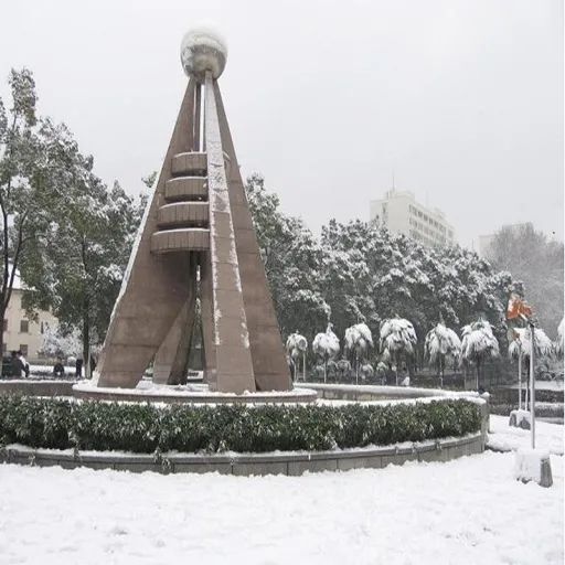
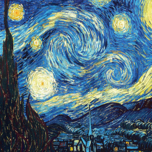
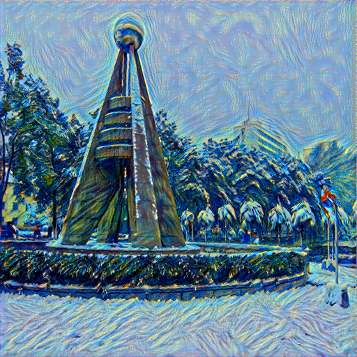
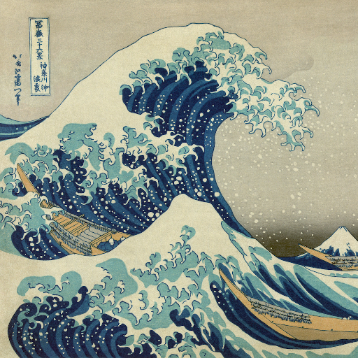
本文主要向大家分享一個小編剛剛學習的神經(jīng)網(wǎng)絡應用的實例：風格遷移(Neural-Transfer)。這是一個由 Leon A. Gatys，Alexander S. Ecker和Matthias Bethge提出的算法。通過這個算法，我們可以用一種新的風格對指定圖片進行重構(gòu)，更通俗一點即：風格圖片+內(nèi)容圖片=輸出圖片，即：

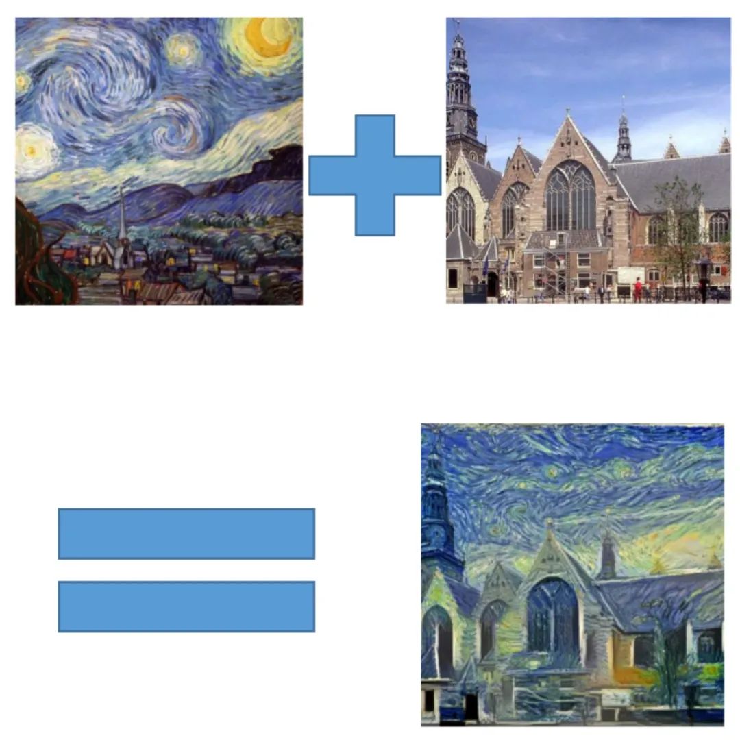
如上圖所示，神經(jīng)風格遷移可以將內(nèi)容圖像的內(nèi)容、風格圖像的風格混合在一起，使得輸出的圖片看起來像內(nèi)容圖像，但采用了風格圖像的風格。這就生成了一個帶有《星空》風格的風景圖，是不是很有趣呢？下面讓我們一起來看看它是怎么實現(xiàn)的吧！

基本原理

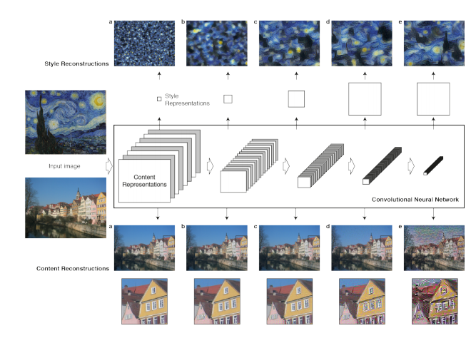
原理很簡單：我們定義了兩個距離，一個為內(nèi)容D_c和一個用于樣式D_s。D_c 測量兩個圖像之間的內(nèi)容有多大不同，而?D_s衡量兩個圖像之間風格的差異。然后，我們生成第三張圖片，并利用D_c和D_s來優(yōu)化這張圖片，使其與內(nèi)容圖片的內(nèi)容差別和風格圖片的風格差別最小化。當然，我們的第一步是利用卷積神經(jīng)網(wǎng)絡提取出圖片的特征，如圖所示：

讀入圖片

現(xiàn)在我們導入content和style的原圖，我們需要使用PIL中的Image來讀取內(nèi)存中的圖片（PS：opencv也可以，但PIL的效果更好一點），再用torchvision中的transforms將讀入圖片轉(zhuǎn)化為tensor以便之后的操作。另外，我們還需要定義一個用于輸出圖像的函數(shù)，以便輸出最終所得到的圖片，該函數(shù)會將tensor轉(zhuǎn)化為圖像。

代碼如下：

# load_img模塊import PIL.Image as Imageimport torchimport torchvision.transforms as transforms
img_size = 512 if torch.cuda.is_available() else 128#根據(jù)設備選擇改變后項數(shù)大小def load_img(img_path):#圖像讀入 ? ?img = Image.open(img_path).convert('RGB')#將圖像讀入并轉(zhuǎn)換成RGB形式 ? ?img = img.resize(img_size, img_size)#調(diào)整讀入圖像像素大小 ? ?img = transforms.ToTensor()(img)#將圖像轉(zhuǎn)化為tensor ? ?img = img.unsqueeze(0)#在0維上增加一個維度 ? ?return img
def show_img(img):#圖像輸出 ? ?img = img.squeeze(0)#將多余的0維通道刪去 ? ?img = transforms.ToPILImage()(img)#將tensor轉(zhuǎn)化為圖像 ? ?img.show()

損失函數(shù)

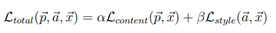
下一步是定義我們的損失函數(shù)，為了實現(xiàn)神經(jīng)風格遷移，我們需要定義一個關于生成圖像（Generated image）G的損失函數(shù)，用于評價生成圖像的好壞。通過最小化損失函數(shù)的方式，來生成所要的圖像。損失函數(shù)需要分成兩部分，一個是內(nèi)容損失函數(shù)，它是關于生成圖像G與內(nèi)容圖像C的函數(shù)，用于衡量生成圖像與內(nèi)容圖像在內(nèi)容上有多相似；一個是風格損失函數(shù)，關于生成圖像G與風格圖像S的函數(shù)，用于衡量生成圖像與風格圖像在風格上的相似度。最后需要用兩個超參數(shù)α和β來確定兩個函數(shù)之間的權(quán)重，我們的總損失是它們兩個的加權(quán)和，即

那么我們的關鍵就在于先單獨求出內(nèi)容損失和風格損失，計算它們的損失也很簡單，首先我們看一下內(nèi)容損失，我們使用最簡單的均方誤差：

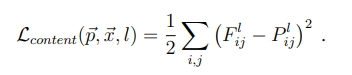
上式是內(nèi)容損失函數(shù)的定義。其中l(wèi)代表第l層的特征表示，p是原始內(nèi)容圖片特征圖，x是生成圖片特征圖。公式的含義就是對于每一層，原始圖片的特征圖（feature map）和生成圖片的特征圖的一一對應做差值平方和。

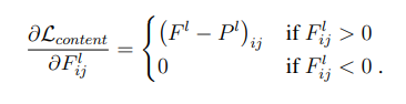
然后我們需要對損失梯度下降求導來優(yōu)化參數(shù)

對于風格損失我們還需要引入Gram矩陣來幫助我們表示圖像的風格特征，我們讀入圖像卷積層的輸出形狀為C × H × W ，C是卷積核的通道數(shù)，每個卷積核學習圖像不同特征，每個卷積核輸出H × W 代表這張圖像的一個feature map，讀入RGB圖像的三色通道相當于三個feature map，我們用Gram矩陣來計算feature map間的相似性，得到圖像的風格特征。

關于Gram矩陣

由于計算風格損失需要Gram矩陣，所以我們先來了解一下它吧。

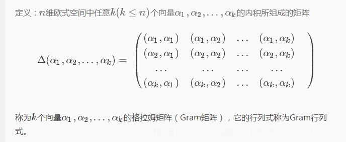
Gram矩陣的定義：

Gram矩陣計算公式：

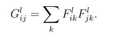
F表示生成圖像的feature map。上面式子的含義：第l層的Gram矩陣第i行，第j列的數(shù)值等于把生成圖像在第l層的第i個feature map與第j個feature map分別拉成一維后相乘求和，即Gram矩陣中的每個值都是每個通道 i 的feature map與每個通道 j 的feature map的內(nèi)積，由于內(nèi)積可以判斷兩個向量之間的夾角和方向關系（如：若a·b>0，則二者方向相同，夾角在0°到90°之間），所以Gram矩陣中的值可以反映出兩個feature map之間的某種關系。

Gram矩陣可以看是feature之間的偏心協(xié)方差矩陣，feature map中的每個數(shù)字都來自于一個特定濾波器在特定位置的卷積，因此每個數(shù)字代表一個特征的強度，而Gram計算的實際上是兩兩特征之間的相關性。Gram的對角線元素提供了不同特征圖各自的信息，而其余元素提供了不同特征圖之間的相關信息，因此，Gram有助于把握整個圖像的大體風格。有了表示風格的Gram矩陣，要度量兩個圖像風格的差異，只需比較他們Gram矩陣的差異即可。

然后我們就可以利用Gram矩陣提取的風格特征計算損失了，這里我們?nèi)匀皇褂镁秸`差，并進行歸一化操作。

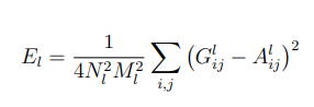
上面是第l層的風格損失函數(shù)，N是指生成圖feature map數(shù)量，M是圖片寬乘高，G是生成圖像的Gram矩陣，A是風格圖像的Gram矩陣。

然后是梯度下降：

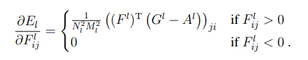
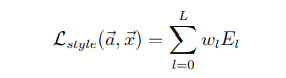
最終的風格損失函數(shù)為每一層的風格損失加權(quán)求和可得。式中，a是指風格圖像，x是指生成圖像，w是指權(quán)重：

下面我們看看如何用代碼實現(xiàn)它：

# loss板塊import torch.nn as nnimport torch
class Content_Loss(nn.Module):#內(nèi)容損失 ? ?def __init__(self, target, weight): ? ? ? ?super(Content_Loss, self).__init__()#繼承父類的初始化 ? ? ? ?self.weight = weight ? ? ? ?self.target = target.detach() * self.weight ? ? ? ?# 必須要用detach來分離出target，這時候target不再是一個Variable，這是為了動態(tài)計算梯度，否則forward會出錯，不能向前傳播 ? ? ? ?self.criterion = nn.MSELoss()#利用均方誤差計算損失 ? ? ? ? ? ?def forward(self, input):#向前計算損失 ? ? ? ?self.loss = self.criterion(input * self.weight, self.target) ? ? ? ?out = input.clone() ? ? ? ?return out ? ? ? ? ? ?def backward(self, retain_graph=True):#反向求導 ? ? ? ?self.loss.backward(retain_graph=retain_graph) ? ? ? ?return self.loss ? ? ? ? ? ? ? ?class Gram(nn.Module):#定義Gram矩陣 ? ?def __init__(self): ? ? ? ?super(Gram, self).__init__() ? ? ? ? ? ?def forward(self, input):#向前計算Gram矩陣 ? ? ? ?a, b, c, d = input.size()#a為批量大小，b為feature map的數(shù)量，c*d為feature map的大小 ? ? ? ?feature = input.view(a * b, c * d) ? ? ? ?gram = torch.mm(feature, feature.t()) ? ? ? ?gram /= (a * b * c * d) ? ? ? ?return gram ? ? ? ? ? ? ? ?class Style_Loss(nn.Module):#風格損失 ? ?def __init__(self, target, weight): ? ? ? ?super(Style_Loss, self).__init__() ? ? ? ?self.weight = weight ? ? ? ?self.target = target.detach() * self.weight ? ? ? ?self.gram = Gram() ? ? ? ?self.criterion = nn.MSELoss() ? ? ? ? ? ?def forward(self, input): ? ? ? ?G = self.gram(input) * self.weight ? ? ? ?self.loss = self.criterion(G, self.target) ? ? ? ?out = input.clone() ? ? ? ?return out ? ? ? ? ? ?def backward(self, retain_graph=True): ? ? ? ?self.loss.backward(retain_graph=retain_graph) ? ? ? ?return self.loss

模型構(gòu)建

接下來就該構(gòu)建我們的模型啦！雖然我們用的是已經(jīng)預訓練好的vgg框架，但我們還需要對它做一些“改造”：把我們之前構(gòu)造好的損失函數(shù)加進去。畢竟“白嫖”也是有限度的嘛！話不多說，上代碼！

# build_model模塊import torch.nn as nnimport torchimport torchvision.models as modelsimport loss ?# 指的是上文中已經(jīng)寫好的loss模塊
device = torch.device("cuda" if torch.cuda.is_available() else "cpu")#選擇運行設備，如果你的電腦有g(shù)pu就在gpu上運行，否則在cpu上運行vgg = models.vgg19(pretrained=True).features.to(device)#這里我們使用預訓練好的vgg19模型'''所需的深度層來計算風格/內(nèi)容損失:'''content_layers_default = ['conv_4']style_layers_default = ['conv_1', 'conv_2', 'conv_3', 'conv_4', 'conv_5']
def get_style_model_and_loss(style_img, ? ? ? ? ? ? ? ? ? ? ? ? ? ? content_img, ? ? ? ? ? ? ? ? ? ? ? ? ? ? cnn=vgg, ? ? ? ? ? ? ? ? ? ? ? ? ? ? style_weight=1000, ? ? ? ? ? ? ? ? ? ? ? ? ? ? content_weight=1, ? ? ? ? ? ? ? ? ? ? ? ? ? ? content_layers=content_layers_default, ? ? ? ? ? ? ? ? ? ? ? ? ? ? style_layers=style_layers_default): ? ?content_loss_list = [] #內(nèi)容損失 ? ?style_loss_list = [] #風格損失 ? ?model = nn.Sequential() #創(chuàng)建一個model，按順序放入layer ? ?model = model.to(device) ? ?gram = loss.Gram().to(device) ? ? ? ?'''把vgg19中的layer、content_loss以及style_loss按順序加入到model中：''' ? ?i = 1 ? ?for layer in cnn: ? ? ? ?if isinstance(layer, nn.Conv2d): ? ? ? ? ? ?name = 'conv_' + str(i) ? ? ? ? ? ?model.add_module(name, layer) ? ? ? ? ? ?if name in content_layers_default: ? ? ? ? ? ? ? ?target = model(content_img) ? ? ? ? ? ? ? ?content_loss = loss.Content_Loss(target, content_weight) ? ? ? ? ? ? ? ?model.add_module('content_loss_' + str(i), content_loss) ? ? ? ? ? ? ? ?content_loss_list.append(content_loss) ? ? ? ? ? ?if name in style_layers_default: ? ? ? ? ? ? ? ?target = model(style_img) ? ? ? ? ? ? ? ?target = gram(target) ? ? ? ? ? ? ? ?style_loss = loss.Style_Loss(target, style_weight) ? ? ? ? ? ? ? ?model.add_module('style_loss_' + str(i), style_loss) ? ? ? ? ? ? ? ?style_loss_list.append(style_loss) ? ? ? ? ? ?i += 1 ? ? ? ?if isinstance(layer, nn.MaxPool2d): ? ? ? ? ? ?name = 'pool_' + str(i) ? ? ? ? ? ?model.add_module(name, layer) ? ? ? ?if isinstance(layer, nn.ReLU): ? ? ? ? ? ?name = 'relu' + str(i) ? ? ? ? ? ?model.add_module(name, layer) ? ? ? ? ? ? ? ?return model, style_loss_list, content_loss_list

執(zhí)行

一切工作準備就緒，我們就可以開始定義我們的run_code模塊了，經(jīng)歷過這么多操作終于走到了最后一步，是不是有點小激動呢？我們的執(zhí)行模塊也很簡單，先定義一個LBFGS優(yōu)化器，然后就可以開始我們一次一次的訓練了。這里我們定義每訓練50次輸出一次我們的損失來評估學習效果。

# run_code模塊import torch.nn as nnimport torch.optim as optimfrom build_model import get_style_model_and_loss
def get_input_param_optimier(input_img): ? ?"""input_img is a Variable""" ? ?input_param = nn.Parameter(input_img.data)#獲取參數(shù) ? ?optimizer = optim.LBFGS([input_param])#用LBFGS優(yōu)化參數(shù) ? ?return input_param, optimizer ? ?def run_style_transfer(content_img, style_img, input_img, num_epoches=300): ? ?print('Building the style transfer model..') ? ?model, style_loss_list, content_loss_list = get_style_model_and_loss( ? ? ? ?style_img, content_img) ? ?input_param, optimizer = get_input_param_optimier(input_img) ? ?print('Opimizing...') ? ?epoch = [0] ? ?while epoch[0] < num_epoches:#每隔50次輸出一次loss ? ? ? ?def closure(): ? ? ? ? ? ?input_param.data.clamp_(0, 1)#修正輸入圖像的值 ? ? ? ? ? ?model(input_param) ? ? ? ? ? ?style_score = 0 ? ? ? ? ? ?content_score = 0 ? ? ? ? ? ?optimizer.zero_grad() ? ? ? ? ? ?for sl in style_loss_list: ? ? ? ? ? ? ? ?style_score += sl.backward() ? ? ? ? ? ?for cl in content_loss_list: ? ? ? ? ? ? ? ?content_score += cl.backward() ? ? ? ? ? ?epoch[0] += 1 ? ? ? ? ? ?if epoch[0] % 50 == 0: ? ? ? ? ? ? ? ?print('run {}'.format(epoch)) ? ? ? ? ? ? ? ?print('Style Loss: {:.4f} Content Loss: {:.4f}'.format( ? ? ? ? ? ? ? ? ? ?style_score.item(), content_score.item())) ? ? ? ? ? ? ? ?print() ? ? ? ? ? ?return style_score + content_score ? ? ? ?optimizer.step(closure) ? ? ? ?input_param.data.clamp_(0, 1)#再次修正 ? ?return input_param.data

運行

最最最最最激動人心的時刻就要到了！敲了這么多代碼，現(xiàn)在我們就可以開始驗證我們的成果了！現(xiàn)在我們只需要挑選一張中意的圖片，再為它尋找一個你想要的風格圖片，只需短短幾分鐘（甚至幾十秒），你，就創(chuàng)造出了屬于自己的藝術(shù)畫作（其實一般）！！！

# start模塊from torch.autograd import Variablefrom torchvision import transformsimport torchfrom run_code import run_style_transferfrom load_img import load_img, show_img
device = torch.device("cuda" if torch.cuda.is_available() else "cpu")style_img = load_img('./picture/style1.png')#風格圖片地址style_img = Variable(style_img).to(device)content_img = load_img('./picture/content5.png')#內(nèi)容圖片地址content_img = Variable(content_img).to(device)input_img = content_img.clone()
out = run_style_transfer(content_img, style_img, input_img, num_epoches=200)#進行200次訓練save_pic = transforms.ToPILImage()(out.cpu().squeeze(0))save_pic.save('./picture/result4.png')#選擇你要保存的地址save_pic.show()

下面我們做幾組演示：

輸入：

輸出：

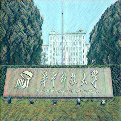
輸入：

輸出：

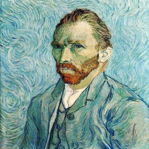
最后我們試一試人像：

輸出：

下面是其中一組loss的輸出：

Opimizing...run [50]Style Loss: 0.7299 Content Loss: 3.7480run [100]Style Loss: 0.3702 Content Loss: 3.3560run [150]Style Loss: 0.2747 Content Loss: 3.1843run [200]Style Loss: 0.2058 Content Loss: 3.0981

我們可以看出內(nèi)容損失還是挺大的，損失的大小不僅跟我們的模型有關，我們選擇的圖片也會對損失有很大的影響，不得不說有的圖片特征確實難以捕獲，小編曾經(jīng)還有過訓練1000次仍然有40多損失的慘痛經(jīng)歷，這種情況就不是單純增加訓練次數(shù)就能解決的了，我們需要更強大的模型去捕獲信息，大家也可以自己試試改進一下模型，也許會有意外的收獲呦！

reference

1] Gatys L A, Ecker A S, Bethge M. A neural algorithm of artistic style[J]. arXiv preprint arXiv:1508.06576, 2015.

2] https://pytorch.org/tutorials/advanced/neural_style_tutorial.html#importing-packages-and-selecting-a-device

END

文案&排版：王心怡（華中科技大學管理學院本科一年級）

? ? ? ? ? ? ? ? ? ? 潘云飛（華中科技大學管理學院本科一年級）

指導老師：秦虎老師（華中科技大學管理學院）

審稿：張宇（華中科技大學管理學院本科二年級）

如對文中內(nèi)容有疑問，歡迎交流。PS：部分資料來自網(wǎng)絡。

如有需求，可以聯(lián)系：

秦虎老師（華中科技大學管理學院：[email protected]）

王心怡（華中科技大學管理學院本科一年級：[email protected]）

潘云飛（華中科技大學管理學院本科一年級：[email protected]）

張宇（華中科技大學管理學院本科二年級：[email protected]）

使用Pytorch實現(xiàn)風格遷移(Neural-Transfer)