機(jī)器學(xué)習(xí)模型評(píng)估與超參數(shù)調(diào)優(yōu)詳解

↑↑↑關(guān)注后"星標(biāo)"Datawhale

每日干貨 &?每月組隊(duì)學(xué)習(xí)，不錯(cuò)過(guò)

?Datawhale干貨?

作者：李祖賢? 深圳大學(xué)，Datawhale高校群成員

機(jī)器學(xué)習(xí)分為兩類(lèi)基本問(wèn)題----回歸與分類(lèi)。在之前的文章中，也介紹了很多基本的機(jī)器學(xué)習(xí)模型。可在Datawhale機(jī)器學(xué)習(xí)專(zhuān)輯中查看。但是，當(dāng)我們建立好了相關(guān)模型以后我們?cè)趺丛u(píng)價(jià)我們建立的模型的好壞以及優(yōu)化我們建立的模型呢？那本次分享的內(nèi)容就是關(guān)于機(jī)器學(xué)習(xí)模型評(píng)估與超參數(shù)調(diào)優(yōu)的。本次分享的內(nèi)容包括：

• 用管道簡(jiǎn)化工作流

• 使用k折交叉驗(yàn)證評(píng)估模型性能

• 使用學(xué)習(xí)和驗(yàn)證曲線調(diào)試算法

• 通過(guò)網(wǎng)格搜索進(jìn)行超參數(shù)調(diào)優(yōu)

• 比較不同的性能評(píng)估指標(biāo)

一、用管道簡(jiǎn)化工作流在很多機(jī)器學(xué)習(xí)算法中，我們可能需要做一系列的基本操作后才能進(jìn)行建模，如：在建立邏輯回歸之前，我們可能需要先對(duì)數(shù)據(jù)進(jìn)行標(biāo)準(zhǔn)化，然后使用PCA將維，最后擬合邏輯回歸模型并預(yù)測(cè)。那有沒(méi)有什么辦法可以同時(shí)進(jìn)行這些操作，使得這些操作形成一個(gè)工作流呢？下面請(qǐng)看代碼：

1. 加載基本工具庫(kù)

import numpy as npimport pandas as pdimport matplotlib.pyplot as plt%matplotlib inlineplt.style.use("ggplot")import warningswarnings.filterwarnings("ignore")

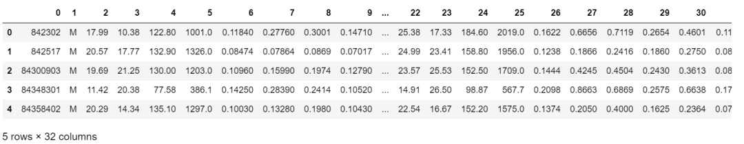
2. 加載數(shù)據(jù)，并做基本預(yù)處理

# 加載數(shù)據(jù)df = pd.read_csv("http://archive.ics.uci.edu/ml/machine-learning-databases/breast-cancer-wisconsin/wdbc.data",header=None)# 做基本的數(shù)據(jù)預(yù)處理from sklearn.preprocessing import LabelEncoder
X = df.iloc[:,2:].valuesy = df.iloc[:,1].valuesle = LabelEncoder()    #將M-B等字符串編碼成計(jì)算機(jī)能識(shí)別的0-1y = le.fit_transform(y)le.transform(['M','B'])# 數(shù)據(jù)切分8：2from sklearn.model_selection import train_test_split
X_train,X_test,y_train,y_test = train_test_split(X,y,test_size=0.2,stratify=y,random_state=1)

3. 把所有的操作全部封在一個(gè)管道pipeline內(nèi)形成一個(gè)工作流：標(biāo)準(zhǔn)化+PCA+邏輯回歸

完成以上操作，共有兩種方式：

方式1：make_pipeline

# 把所有的操作全部封在一個(gè)管道pipeline內(nèi)形成一個(gè)工作流：##?標(biāo)準(zhǔn)化+PCA+邏輯回歸
### 方式1：make_pipelinefrom sklearn.preprocessing import StandardScalerfrom sklearn.decomposition import PCAfrom sklearn.linear_model import LogisticRegressionfrom sklearn.pipeline import make_pipeline
pipe_lr1 = make_pipeline(StandardScaler(),PCA(n_components=2),LogisticRegression(random_state=1))pipe_lr1.fit(X_train,y_train)y_pred1 = pipe_lr.predict(X_test)print("Test?Accuracy:?%.3f"%?pipe_lr1.score(X_test,y_test))

Test Accuracy: 0.956

方式2：Pipeline

# 把所有的操作全部封在一個(gè)管道pipeline內(nèi)形成一個(gè)工作流：##?標(biāo)準(zhǔn)化+PCA+邏輯回歸
### 方式2：Pipelinefrom sklearn.preprocessing import StandardScalerfrom sklearn.decomposition import PCAfrom sklearn.linear_model import LogisticRegressionfrom sklearn.pipeline import Pipeline
pipe_lr2 = Pipeline([['std',StandardScaler()],['pca',PCA(n_components=2)],['lr',LogisticRegression(random_state=1)]])pipe_lr2.fit(X_train,y_train)y_pred2 = pipe_lr2.predict(X_test)print("Test Accuracy: %.3f"% pipe_lr2.score(X_test,y_test))

Test Accuracy: 0.956

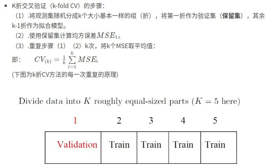
二、使用k折交叉驗(yàn)證評(píng)估模型性能

評(píng)估方式1：k折交叉驗(yàn)證

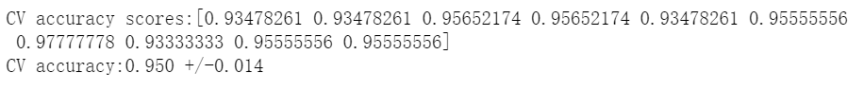
# 評(píng)估方式1：k折交叉驗(yàn)證
from sklearn.model_selection import cross_val_score
scores1 = cross_val_score(estimator=pipe_lr,X = X_train,y = y_train,cv=10,n_jobs=1)print("CV accuracy scores:%s" % scores1)print("CV accuracy:%.3f +/-%.3f"%(np.mean(scores1),np.std(scores1)))

評(píng)估方式2：分層k折交叉驗(yàn)證

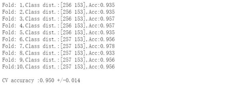
# 評(píng)估方式2：分層k折交叉驗(yàn)證
from sklearn.model_selection import StratifiedKFold
kfold = StratifiedKFold(n_splits=10,random_state=1).split(X_train,y_train)scores2 = []for k,(train,test) in enumerate(kfold):    pipe_lr.fit(X_train[train],y_train[train])    score = pipe_lr.score(X_train[test],y_train[test])    scores2.append(score)    print('Fold:%2d,Class dist.:%s,Acc:%.3f'%(k+1,np.bincount(y_train[train]),score))print('\nCV accuracy :%.3f +/-%.3f'%(np.mean(scores2),np.std(scores2)))

三、?使用學(xué)習(xí)和驗(yàn)證曲線調(diào)試算法

如果模型過(guò)于復(fù)雜，即模型有太多的自由度或者參數(shù)，就會(huì)有過(guò)擬合的風(fēng)險(xiǎn)（高方差）；而模型過(guò)于簡(jiǎn)單，則會(huì)有欠擬合的風(fēng)險(xiǎn)(高偏差)。

下面我們用這些曲線去識(shí)別并解決方差和偏差問(wèn)題：

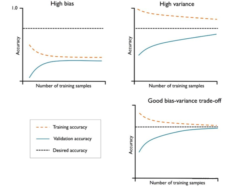
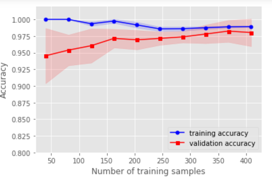
1. 用學(xué)習(xí)曲線診斷偏差與方差

# 用學(xué)習(xí)曲線診斷偏差與方差from sklearn.model_selection import learning_curve
pipe_lr3 = make_pipeline(StandardScaler(),LogisticRegression(random_state=1,penalty='l2'))train_sizes,train_scores,test_scores = learning_curve(estimator=pipe_lr3,X=X_train,y=y_train,train_sizes=np.linspace(0.1,1,10),cv=10,n_jobs=1)train_mean = np.mean(train_scores,axis=1)train_std = np.std(train_scores,axis=1)test_mean = np.mean(test_scores,axis=1)test_std = np.std(test_scores,axis=1)plt.plot(train_sizes,train_mean,color='blue',marker='o',markersize=5,label='training accuracy')plt.fill_between(train_sizes,train_mean+train_std,train_mean-train_std,alpha=0.15,color='blue')plt.plot(train_sizes,test_mean,color='red',marker='s',markersize=5,label='validation accuracy')plt.fill_between(train_sizes,test_mean+test_std,test_mean-test_std,alpha=0.15,color='red')plt.xlabel("Number of training samples")plt.ylabel("Accuracy")plt.legend(loc='lower right')plt.ylim([0.8,1.02])plt.show()

2. 用驗(yàn)證曲線解決欠擬合和過(guò)擬合

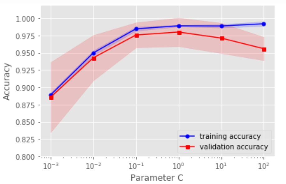
# 用驗(yàn)證曲線解決欠擬合和過(guò)擬合from sklearn.model_selection import validation_curve
pipe_lr3 = make_pipeline(StandardScaler(),LogisticRegression(random_state=1,penalty='l2'))param_range = [0.001,0.01,0.1,1.0,10.0,100.0]train_scores,test_scores = validation_curve(estimator=pipe_lr3,X=X_train,y=y_train,param_name='logisticregression__C',param_range=param_range,cv=10,n_jobs=1)train_mean = np.mean(train_scores,axis=1)train_std = np.std(train_scores,axis=1)test_mean = np.mean(test_scores,axis=1)test_std = np.std(test_scores,axis=1)plt.plot(param_range,train_mean,color='blue',marker='o',markersize=5,label='training accuracy')plt.fill_between(param_range,train_mean+train_std,train_mean-train_std,alpha=0.15,color='blue')plt.plot(param_range,test_mean,color='red',marker='s',markersize=5,label='validation accuracy')plt.fill_between(param_range,test_mean+test_std,test_mean-test_std,alpha=0.15,color='red')plt.xscale('log')plt.xlabel("Parameter C")plt.ylabel("Accuracy")plt.legend(loc='lower right')plt.ylim([0.8,1.02])plt.show()

四、通過(guò)網(wǎng)格搜索進(jìn)行超參數(shù)調(diào)優(yōu)

如果只有一個(gè)參數(shù)需要調(diào)整，那么用驗(yàn)證曲線手動(dòng)調(diào)整是一個(gè)好方法，但是隨著需要調(diào)整的超參數(shù)越來(lái)越多的時(shí)候，我們能不能自動(dòng)去調(diào)整呢？！！！注意對(duì)比各個(gè)算法的時(shí)間復(fù)雜度。

（注意參數(shù)與超參數(shù)的區(qū)別：參數(shù)可以通過(guò)優(yōu)化算法進(jìn)行優(yōu)化，如邏輯回歸的系數(shù)；超參數(shù)是不能用優(yōu)化模型進(jìn)行優(yōu)化的，如正則話的系數(shù)。）

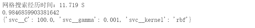
方式1：網(wǎng)格搜索GridSearchCV()

# 方式1：網(wǎng)格搜索GridSearchCV()from sklearn.model_selection import GridSearchCVfrom sklearn.svm import SVCimport time
start_time = time.time()pipe_svc = make_pipeline(StandardScaler(),SVC(random_state=1))param_range = [0.0001,0.001,0.01,0.1,1.0,10.0,100.0,1000.0]param_grid = [{'svc__C':param_range,'svc__kernel':['linear']},{'svc__C':param_range,'svc__gamma':param_range,'svc__kernel':['rbf']}]gs = GridSearchCV(estimator=pipe_svc,param_grid=param_grid,scoring='accuracy',cv=10,n_jobs=-1)gs = gs.fit(X_train,y_train)end_time = time.time()print("網(wǎng)格搜索經(jīng)歷時(shí)間：%.3f S" % float(end_time-start_time))print(gs.best_score_)print(gs.best_params_)

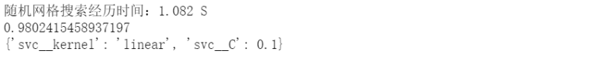
方式2：隨機(jī)網(wǎng)格搜索RandomizedSearchCV()

# 方式2：隨機(jī)網(wǎng)格搜索RandomizedSearchCV()from sklearn.model_selection import RandomizedSearchCVfrom sklearn.svm import SVCimport time
start_time = time.time()pipe_svc = make_pipeline(StandardScaler(),SVC(random_state=1))param_range = [0.0001,0.001,0.01,0.1,1.0,10.0,100.0,1000.0]param_grid = [{'svc__C':param_range,'svc__kernel':['linear']},{'svc__C':param_range,'svc__gamma':param_range,'svc__kernel':['rbf']}]# param_grid = [{'svc__C':param_range,'svc__kernel':['linear','rbf'],'svc__gamma':param_range}]gs = RandomizedSearchCV(estimator=pipe_svc, param_distributions=param_grid,scoring='accuracy',cv=10,n_jobs=-1)gs = gs.fit(X_train,y_train)end_time = time.time()print("隨機(jī)網(wǎng)格搜索經(jīng)歷時(shí)間：%.3f S" % float(end_time-start_time))print(gs.best_score_)print(gs.best_params_)

方式3：嵌套交叉驗(yàn)證

# 方式3：嵌套交叉驗(yàn)證from sklearn.model_selection import GridSearchCVfrom sklearn.svm import SVCfrom sklearn.model_selection import cross_val_scoreimport time
start_time = time.time()pipe_svc = make_pipeline(StandardScaler(),SVC(random_state=1))param_range = [0.0001,0.001,0.01,0.1,1.0,10.0,100.0,1000.0]param_grid = [{'svc__C':param_range,'svc__kernel':['linear']},{'svc__C':param_range,'svc__gamma':param_range,'svc__kernel':['rbf']}]gs = GridSearchCV(estimator=pipe_svc, param_grid=param_grid,scoring='accuracy',cv=2,n_jobs=-1)scores = cross_val_score(gs,X_train,y_train,scoring='accuracy',cv=5)end_time = time.time()print("嵌套交叉驗(yàn)證：%.3f S" % float(end_time-start_time))print('CV accuracy :%.3f +/-%.3f'%(np.mean(scores),np.std(scores)))

五、比較不同的性能評(píng)估指標(biāo)

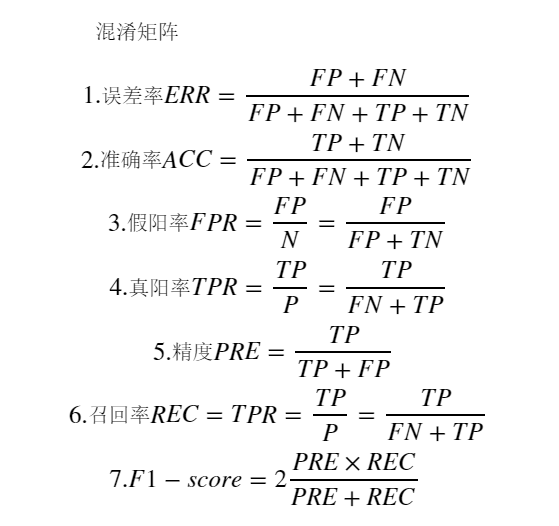
有時(shí)候，準(zhǔn)確率不是我們唯一需要考慮的評(píng)價(jià)指標(biāo)，因?yàn)橛袝r(shí)候會(huì)存在各類(lèi)預(yù)測(cè)錯(cuò)誤的代價(jià)不一樣。例如：在預(yù)測(cè)一個(gè)人的腫瘤疾病的時(shí)候，如果病人A真實(shí)得腫瘤但是我們預(yù)測(cè)他是沒(méi)有腫瘤，跟A真實(shí)是健康但是預(yù)測(cè)他是腫瘤，二者付出的代價(jià)很大區(qū)別（想想為什么）。所以我們需要其他更加廣泛的指標(biāo)：

1. 繪制混淆矩陣

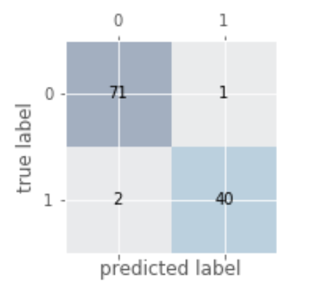
# 繪制混淆矩陣from sklearn.metrics import confusion_matrix
pipe_svc.fit(X_train,y_train)y_pred = pipe_svc.predict(X_test)confmat = confusion_matrix(y_true=y_test,y_pred=y_pred)fig,ax = plt.subplots(figsize=(2.5,2.5))ax.matshow(confmat, cmap=plt.cm.Blues,alpha=0.3)for i in range(confmat.shape[0]):    for j in range(confmat.shape[1]):        ax.text(x=j,y=i,s=confmat[i,j],va='center',ha='center')plt.xlabel('predicted label')plt.ylabel('true label')plt.show()

2. 各種指標(biāo)的計(jì)算

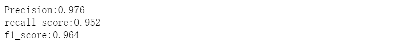
# 各種指標(biāo)的計(jì)算from sklearn.metrics import precision_score,recall_score,f1_score
print('Precision:%.3f'%precision_score(y_true=y_test,y_pred=y_pred))print('recall_score:%.3f'%recall_score(y_true=y_test,y_pred=y_pred))print('f1_score:%.3f'%f1_score(y_true=y_test,y_pred=y_pred))

3. 將不同的指標(biāo)與GridSearch結(jié)合

# 將不同的指標(biāo)與GridSearch結(jié)合from sklearn.metrics import make_scorer,f1_scorescorer = make_scorer(f1_score,pos_label=0)gs = GridSearchCV(estimator=pipe_svc,param_grid=param_grid,scoring=scorer,cv=10)gs = gs.fit(X_train,y_train)print(gs.best_score_)print(gs.best_params_)

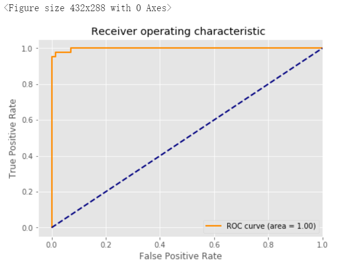
4. 繪制ROC曲線

# 繪制ROC曲線from sklearn.metrics import roc_curve,aucfrom sklearn.metrics import make_scorer,f1_scorescorer = make_scorer(f1_score,pos_label=0)gs = GridSearchCV(estimator=pipe_svc,param_grid=param_grid,scoring=scorer,cv=10)y_pred = gs.fit(X_train,y_train).decision_function(X_test)#y_pred = gs.predict(X_test)fpr,tpr,threshold = roc_curve(y_test, y_pred) ###計(jì)算真陽(yáng)率和假陽(yáng)率roc_auc = auc(fpr,tpr) ###計(jì)算auc的值plt.figure()lw = 2plt.figure(figsize=(7,5))plt.plot(fpr, tpr, color='darkorange',         lw=lw, label='ROC curve (area = %0.2f)' % roc_auc) ###假陽(yáng)率為橫坐標(biāo)，真陽(yáng)率為縱坐標(biāo)做曲線plt.plot([0, 1], [0, 1], color='navy', lw=lw, linestyle='--')plt.xlim([-0.05, 1.0])plt.ylim([-0.05, 1.05])plt.xlabel('False Positive Rate')plt.ylabel('True Positive Rate')plt.title('Receiver operating characteristic ')plt.legend(loc="lower right")plt.show()

本文電子版及代碼源文件 后臺(tái)回復(fù) 模型評(píng)估 獲取

“感謝你的分享，點(diǎn)贊，在看三連↓