熱文 | 卷積神經(jīng)網(wǎng)絡(luò)入門案例，輕松實現(xiàn)花朵分類

# 下載數(shù)據(jù)集
import pathlib
dataset_url = "https://storage.googleapis.com/download.tensorflow.org/example_images/flower_photos.tgz"
data_dir = tf.keras.utils.get_file('flower_photos', origin=dataset_url, untar=True)
data_dir = pathlib.Path(data_dir)

# 查看數(shù)據(jù)集圖片的總數(shù)量
image_count = len(list(data_dir.glob('*/*.jpg')))
print(image_count)

# 查看郁金香tulips目錄下的第1張圖片；
tulips = list(data_dir.glob('tulips/*'))
PIL.Image.open(str(tulips[0]))

# 定義加載圖片的一些參數(shù)，包括：批量大小、圖像高度、圖像寬度
batch_size = 32
img_height = 180
img_width = 180

# 將80％的圖像用于訓(xùn)練
train_ds = tf.keras.preprocessing.image_dataset_from_directory(
  data_dir,
  validation_split=0.2,
  subset="training",
  seed=123,
  image_size=(img_height, img_width),
  batch_size=batch_size)

# 將20％的圖像用于驗證
val_ds = tf.keras.preprocessing.image_dataset_from_directory(
  data_dir,
  validation_split=0.2,
  subset="validation",
  seed=123,
  image_size=(img_height, img_width),
  batch_size=batch_size)

# 打印數(shù)據(jù)集中花朵的類別名稱，字母順序?qū)?yīng)于目錄名稱
class_names = train_ds.class_names
print(class_names)

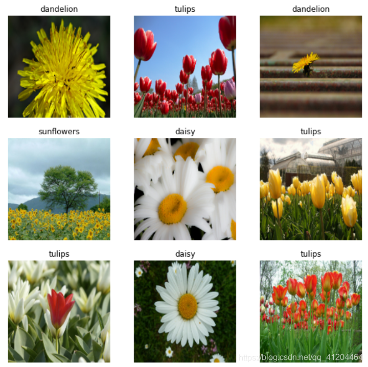
# 查看一下訓(xùn)練數(shù)據(jù)集中的9張圖像
import matplotlib.pyplot as plt

plt.figure(figsize=(10, 10))
for images, labels in train_ds.take(1):
  for i in range(9):
    ax = plt.subplot(3, 3, i + 1)
    plt.imshow(images[i].numpy().astype("uint8"))
    plt.title(class_names[labels[i]])
    plt.axis("off")

for image_batch, labels_batch in train_ds:
  print(image_batch.shape)
  print(labels_batch.shape)
  break

# 將像素的值標準化至0到1的區(qū)間內(nèi)。
normalization_layer = layers.experimental.preprocessing.Rescaling(1./255)

# 調(diào)用map將其應(yīng)用于數(shù)據(jù)集：
normalized_ds = train_ds.map(lambda x, y: (normalization_layer(x), y))
image_batch, labels_batch = next(iter(normalized_ds))
first_image = image_batch[0]
# Notice the pixels values are now in `[0,1]`.
print(np.min(first_image), np.max(first_image))

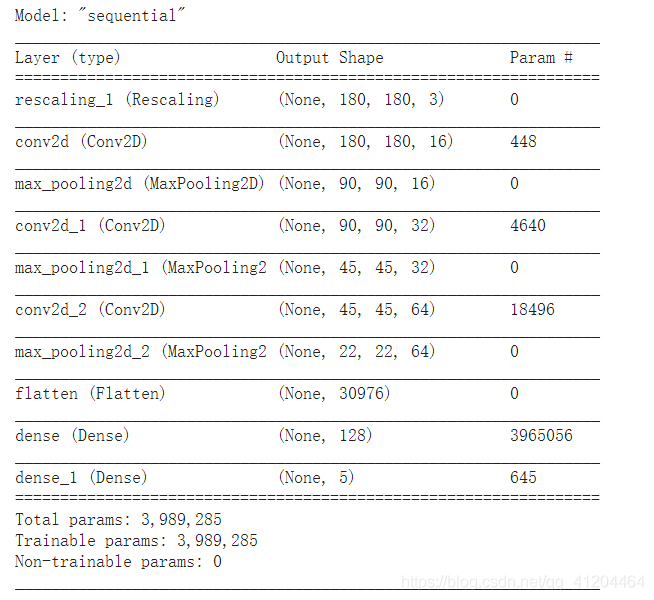
num_classes = 5

model = Sequential([
  layers.experimental.preprocessing.Rescaling(1./255, input_shape=(img_height, img_width, 3)),
  layers.Conv2D(16, 3, padding='same', activation='relu'),
  layers.MaxPooling2D(),
  layers.Conv2D(32, 3, padding='same', activation='relu'),
  layers.MaxPooling2D(),
  layers.Conv2D(64, 3, padding='same', activation='relu'),
  layers.MaxPooling2D(),
  layers.Flatten(),
  layers.Dense(128, activation='relu'),
  layers.Dense(num_classes)
])

model.compile(optimizer='adam',
              loss=tf.keras.losses.SparseCategoricalCrossentropy(from_logits=True),
              metrics=['accuracy'])

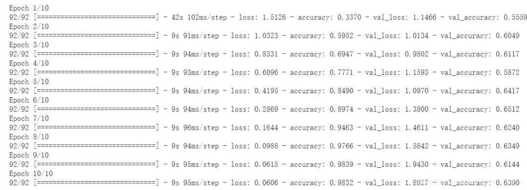
epochs=10
history = model.fit(
  train_ds,
  validation_data=val_ds,
  epochs=epochs
)

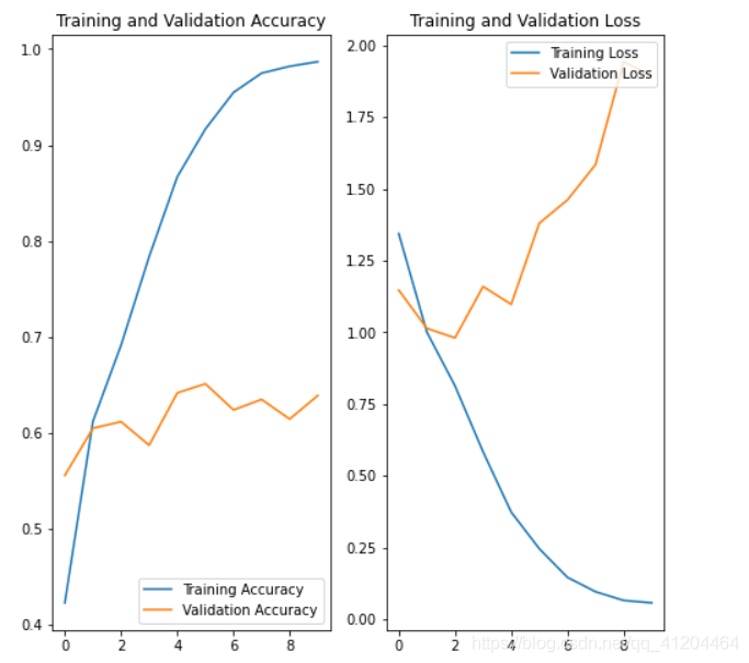
acc = history.history['accuracy']
val_acc = history.history['val_accuracy']

loss = history.history['loss']
val_loss = history.history['val_loss']

epochs_range = range(epochs)

plt.figure(figsize=(8, 8))
plt.subplot(1, 2, 1)
plt.plot(epochs_range, acc, label='Training Accuracy')
plt.plot(epochs_range, val_acc, label='Validation Accuracy')
plt.legend(loc='lower right')
plt.title('Training and Validation Accuracy')

plt.subplot(1, 2, 2)
plt.plot(epochs_range, loss, label='Training Loss')
plt.plot(epochs_range, val_loss, label='Validation Loss')
plt.legend(loc='upper right')
plt.title('Training and Validation Loss')
plt.show()

data_augmentation = keras.Sequential(
  [
    layers.experimental.preprocessing.RandomFlip("horizontal", 
                                                 input_shape=(img_height, 
                                                              img_width,
                                                              3)),
    layers.experimental.preprocessing.RandomRotation(0.1),
    layers.experimental.preprocessing.RandomZoom(0.1),
  ]
)

plt.figure(figsize=(10, 10))
for images, _ in train_ds.take(1):
  for i in range(9):
    augmented_images = data_augmentation(images)
    ax = plt.subplot(3, 3, i + 1)
    plt.imshow(augmented_images[0].numpy().astype("uint8"))
    plt.axis("off")

model = Sequential([
  data_augmentation,
  layers.experimental.preprocessing.Rescaling(1./255),
  layers.Conv2D(16, 3, padding='same', activation='relu'),
  layers.MaxPooling2D(),
  layers.Conv2D(32, 3, padding='same', activation='relu'),
  layers.MaxPooling2D(),
  layers.Conv2D(64, 3, padding='same', activation='relu'),
  layers.MaxPooling2D(),
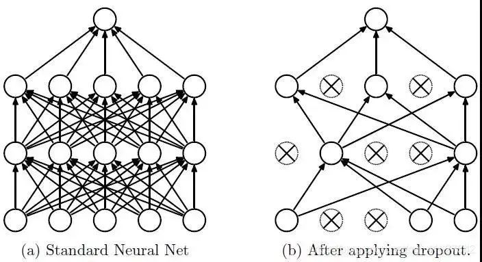
  layers.Dropout(0.2),
  layers.Flatten(),
  layers.Dense(128, activation='relu'),
  layers.Dense(num_classes)
])

# 編譯模型
model.compile(optimizer='adam',
              loss=tf.keras.losses.SparseCategoricalCrossentropy(from_logits=True),
              metrics=['accuracy'])
# 查看網(wǎng)絡(luò)結(jié)構(gòu)
model.summary()
# 訓(xùn)練模型
epochs = 15
history = model.fit(
  train_ds,
  validation_data=val_ds,
  epochs=epochs
)

acc = history.history['accuracy']
val_acc = history.history['val_accuracy']

loss = history.history['loss']
val_loss = history.history['val_loss']

epochs_range = range(epochs)

plt.figure(figsize=(8, 8))
plt.subplot(1, 2, 1)
plt.plot(epochs_range, acc, label='Training Accuracy')
plt.plot(epochs_range, val_acc, label='Validation Accuracy')
plt.legend(loc='lower right')
plt.title('Training and Validation Accuracy')

plt.subplot(1, 2, 2)
plt.plot(epochs_range, loss, label='Training Loss')
plt.plot(epochs_range, val_loss, label='Validation Loss')
plt.legend(loc='upper right')
plt.title('Training and Validation Loss')
plt.show()

# 預(yù)測新數(shù)據(jù) 下載一張新圖片，來預(yù)測它屬于什么類型花朵
sunflower_url = "https://storage.googleapis.com/download.tensorflow.org/example_images/592px-Red_sunflower.jpg"
sunflower_path = tf.keras.utils.get_file('Red_sunflower', origin=sunflower_url)

img = keras.preprocessing.image.load_img(
    sunflower_path, target_size=(img_height, img_width)
)
img_array = keras.preprocessing.image.img_to_array(img)
img_array = tf.expand_dims(img_array, 0) # Create a batch

predictions = model.predict(img_array)
score = tf.nn.softmax(predictions[0])

print(
    "該圖像最有可能屬于{}，置信度為 {:.2f}%"
    .format(class_names[np.argmax(score)], 100 * np.max(score))
)

'''
環(huán)境：Tensorflow2  Python3.x
'''

import matplotlib.pyplot as plt
import numpy as np
import os
import PIL
import tensorflow as tf

from tensorflow import keras
from tensorflow.keras import layers
from tensorflow.keras.models import Sequential

# 下載數(shù)據(jù)集
import pathlib
dataset_url = "https://storage.googleapis.com/download.tensorflow.org/example_images/flower_photos.tgz"
data_dir = tf.keras.utils.get_file('flower_photos', origin=dataset_url, untar=True)
data_dir = pathlib.Path(data_dir)

# 查看數(shù)據(jù)集圖片的總數(shù)量
image_count = len(list(data_dir.glob('*/*.jpg')))
print(image_count)

# 查看郁金香tulips目錄下的第1張圖片；
tulips = list(data_dir.glob('tulips/*'))
PIL.Image.open(str(tulips[0]))

# 定義加載圖片的一些參數(shù)，包括：批量大小、圖像高度、圖像寬度
batch_size = 32
img_height = 180
img_width = 180

# 將80％的圖像用于訓(xùn)練
train_ds = tf.keras.preprocessing.image_dataset_from_directory(
  data_dir,
  validation_split=0.2,
  subset="training",
  seed=123,
  image_size=(img_height, img_width),
  batch_size=batch_size)

# 將20％的圖像用于驗證
val_ds = tf.keras.preprocessing.image_dataset_from_directory(
  data_dir,
  validation_split=0.2,
  subset="validation",
  seed=123,
  image_size=(img_height, img_width),
  batch_size=batch_size)

# 打印數(shù)據(jù)集中花朵的類別名稱，字母順序?qū)?yīng)于目錄名稱
class_names = train_ds.class_names
print(class_names)


# 將像素的值標準化至0到1的區(qū)間內(nèi)。
normalization_layer = layers.experimental.preprocessing.Rescaling(1./255)

# 調(diào)用map將其應(yīng)用于數(shù)據(jù)集：
normalized_ds = train_ds.map(lambda x, y: (normalization_layer(x), y))
image_batch, labels_batch = next(iter(normalized_ds))
first_image = image_batch[0]
# Notice the pixels values are now in `[0,1]`.
print(np.min(first_image), np.max(first_image))

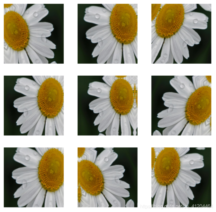
# 數(shù)據(jù)增強 通過對已有的訓(xùn)練集圖片 隨機轉(zhuǎn)換（反轉(zhuǎn)、旋轉(zhuǎn)、縮放等），來生成其它訓(xùn)練數(shù)據(jù)
data_augmentation = keras.Sequential(
  [
    layers.experimental.preprocessing.RandomFlip("horizontal", 
                                                 input_shape=(img_height, 
                                                              img_width,
                                                              3)),
    layers.experimental.preprocessing.RandomRotation(0.1),
    layers.experimental.preprocessing.RandomZoom(0.1),
  ]
)

# 搭建 網(wǎng)絡(luò)模型
model = Sequential([
  data_augmentation,
  layers.experimental.preprocessing.Rescaling(1./255),
  layers.Conv2D(16, 3, padding='same', activation='relu'),
  layers.MaxPooling2D(),
  layers.Conv2D(32, 3, padding='same', activation='relu'),
  layers.MaxPooling2D(),
  layers.Conv2D(64, 3, padding='same', activation='relu'),
  layers.MaxPooling2D(),
  layers.Dropout(0.2),
  layers.Flatten(),
  layers.Dense(128, activation='relu'),
  layers.Dense(num_classes)
])

# 編譯模型
model.compile(optimizer='adam',
              loss=tf.keras.losses.SparseCategoricalCrossentropy(from_logits=True),
              metrics=['accuracy'])

# 查看網(wǎng)絡(luò)結(jié)構(gòu)
model.summary()

# 訓(xùn)練模型
epochs = 15
history = model.fit(
  train_ds,
  validation_data=val_ds,
  epochs=epochs
)

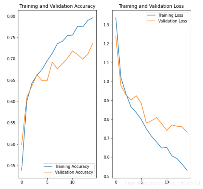
# 在訓(xùn)練和驗證集上查看損失值和準確性
acc = history.history['accuracy']
val_acc = history.history['val_accuracy']

loss = history.history['loss']
val_loss = history.history['val_loss']

epochs_range = range(epochs)

plt.figure(figsize=(8, 8))
plt.subplot(1, 2, 1)
plt.plot(epochs_range, acc, label='Training Accuracy')
plt.plot(epochs_range, val_acc, label='Validation Accuracy')
plt.legend(loc='lower right')
plt.title('Training and Validation Accuracy')

plt.subplot(1, 2, 2)
plt.plot(epochs_range, loss, label='Training Loss')
plt.plot(epochs_range, val_loss, label='Validation Loss')
plt.legend(loc='upper right')
plt.title('Training and Validation Loss')
plt.show()