
10種聚類算法的完整python操作示例
聚類或聚類分析是無監(jiān)督學(xué)習(xí)問題。它通常被用作數(shù)據(jù)分析技術(shù),用于發(fā)現(xiàn)數(shù)據(jù)中的有趣模式,例如基于其行為的客戶群。有許多聚類算法可供選擇,對(duì)于所有情況,沒有單一的最佳聚類算法。相反,最好探索一系列聚類算法以及每種算法的不同配置。在本教程中,你將發(fā)現(xiàn)如何在 python 中安裝和使用頂級(jí)聚類算法。
完成本教程后,你將知道:
聚類是在輸入數(shù)據(jù)的特征空間中查找自然組的無監(jiān)督問題。
對(duì)于所有數(shù)據(jù)集,有許多不同的聚類算法和單一的最佳方法。
在 scikit-learn 機(jī)器學(xué)習(xí)庫的 Python 中如何實(shí)現(xiàn)、適配和使用頂級(jí)聚類算法。
讓我們開始吧。
教程概述
本教程分為三部分:
聚類
聚類算法
聚類算法示例
庫安裝
聚類數(shù)據(jù)集
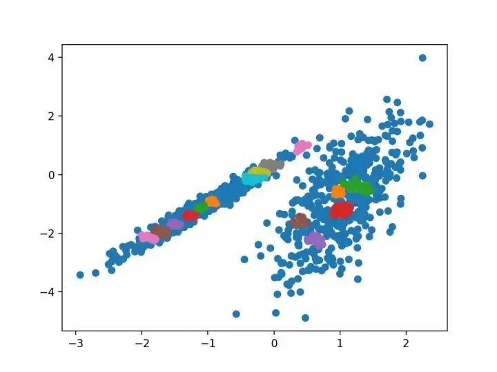
親和力傳播
聚合聚類
BIRCH
DBSCAN
K-均值
Mini-Batch K-均值
Mean Shift
OPTICS
光譜聚類
高斯混合模型
聚類技術(shù)適用于沒有要預(yù)測(cè)的類,而是將實(shí)例劃分為自然組的情況。
—源自:《數(shù)據(jù)挖掘頁:實(shí)用機(jī)器學(xué)習(xí)工具和技術(shù)》2016年。
這些群集可能反映出在從中繪制實(shí)例的域中工作的某種機(jī)制,這種機(jī)制使某些實(shí)例彼此具有比它們與其余實(shí)例更強(qiáng)的相似性。
—源自:《數(shù)據(jù)挖掘頁:實(shí)用機(jī)器學(xué)習(xí)工具和技術(shù)》2016年。
該進(jìn)化樹可以被認(rèn)為是人工聚類分析的結(jié)果; 將正常數(shù)據(jù)與異常值或異常分開可能會(huì)被認(rèn)為是聚類問題; 根據(jù)自然行為將集群分開是一個(gè)集群?jiǎn)栴},稱為市場(chǎng)細(xì)分。
聚類是一種無監(jiān)督學(xué)習(xí)技術(shù),因此很難評(píng)估任何給定方法的輸出質(zhì)量。
—源自:《機(jī)器學(xué)習(xí)頁:概率觀點(diǎn)》2012。
聚類分析的所有目標(biāo)的核心是被群集的各個(gè)對(duì)象之間的相似程度(或不同程度)的概念。聚類方法嘗試根據(jù)提供給對(duì)象的相似性定義對(duì)對(duì)象進(jìn)行分組。
—源自:《統(tǒng)計(jì)學(xué)習(xí)的要素:數(shù)據(jù)挖掘、推理和預(yù)測(cè)》,2016年
親和力傳播 聚合聚類 BIRCH DBSCAN K-均值 Mini-Batch K-均值 Mean Shift OPTICS 光譜聚類 高斯混合
三.聚類算法示例
sudo pip install scikit-learn
# 檢查 scikit-learn 版本
import sklearn
print(sklearn.__version__)
0.22.1
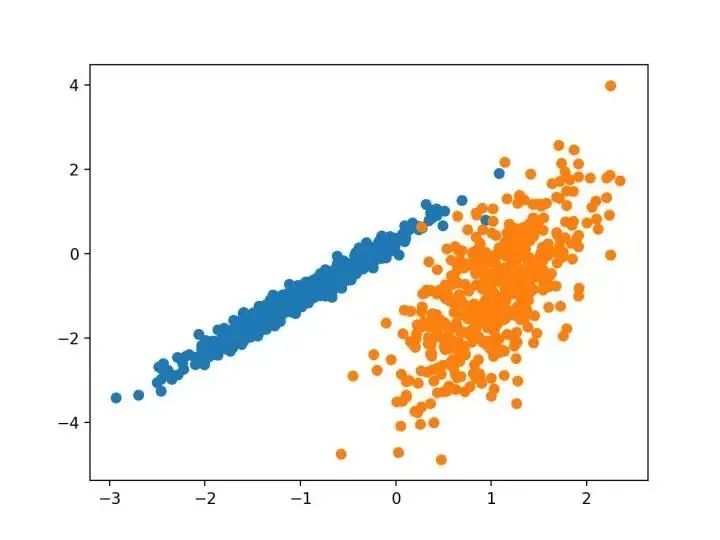
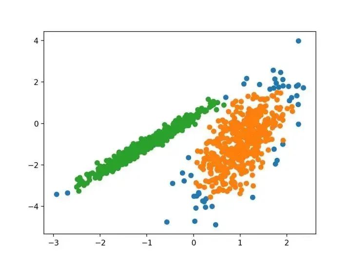
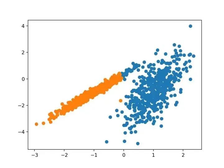
# 綜合分類數(shù)據(jù)集
from numpy import where
from sklearn.datasets import make_classification
from matplotlib import pyplot
# 定義數(shù)據(jù)集
X, y = make_classification(n_samples=1000, n_features=2, n_informative=2, n_redundant=0, n_clusters_per_class=1, random_state=4)
# 為每個(gè)類的樣本創(chuàng)建散點(diǎn)圖
for class_value in range(2):
# 獲取此類的示例的行索引
row_ix = where(y == class_value)
# 創(chuàng)建這些樣本的散布
pyplot.scatter(X[row_ix, 0], X[row_ix, 1])
# 繪制散點(diǎn)圖
pyplot.show()
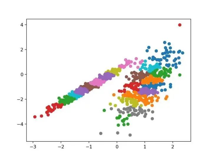
我們?cè)O(shè)計(jì)了一種名為“親和傳播”的方法,它作為兩對(duì)數(shù)據(jù)點(diǎn)之間相似度的輸入度量。在數(shù)據(jù)點(diǎn)之間交換實(shí)值消息,直到一組高質(zhì)量的范例和相應(yīng)的群集逐漸出現(xiàn)
—源自:《通過在數(shù)據(jù)點(diǎn)之間傳遞消息》2007。
# 親和力傳播聚類
from numpy import unique
from numpy import where
from sklearn.datasets import make_classification
from sklearn.cluster import AffinityPropagation
from matplotlib import pyplot
# 定義數(shù)據(jù)集
X, _ = make_classification(n_samples=1000, n_features=2, n_informative=2, n_redundant=0, n_clusters_per_class=1, random_state=4)
# 定義模型
model = AffinityPropagation(damping=0.9)
# 匹配模型
model.fit(X)
# 為每個(gè)示例分配一個(gè)集群
yhat = model.predict(X)
# 檢索唯一群集
clusters = unique(yhat)
# 為每個(gè)群集的樣本創(chuàng)建散點(diǎn)圖
for cluster in clusters:
# 獲取此群集的示例的行索引
row_ix = where(yhat == cluster)
# 創(chuàng)建這些樣本的散布
pyplot.scatter(X[row_ix, 0], X[row_ix, 1])
# 繪制散點(diǎn)圖
pyplot.show()
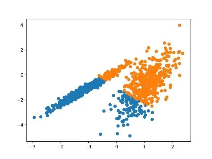
# 聚合聚類
from numpy import unique
from numpy import where
from sklearn.datasets import make_classification
from sklearn.cluster import AgglomerativeClustering
from matplotlib import pyplot
# 定義數(shù)據(jù)集
X, _ = make_classification(n_samples=1000, n_features=2, n_informative=2, n_redundant=0, n_clusters_per_class=1, random_state=4)
# 定義模型
model = AgglomerativeClustering(n_clusters=2)
# 模型擬合與聚類預(yù)測(cè)
yhat = model.fit_predict(X)
# 檢索唯一群集
clusters = unique(yhat)
# 為每個(gè)群集的樣本創(chuàng)建散點(diǎn)圖
for cluster in clusters:
# 獲取此群集的示例的行索引
row_ix = where(yhat == cluster)
# 創(chuàng)建這些樣本的散布
pyplot.scatter(X[row_ix, 0], X[row_ix, 1])
# 繪制散點(diǎn)圖
pyplot.show()
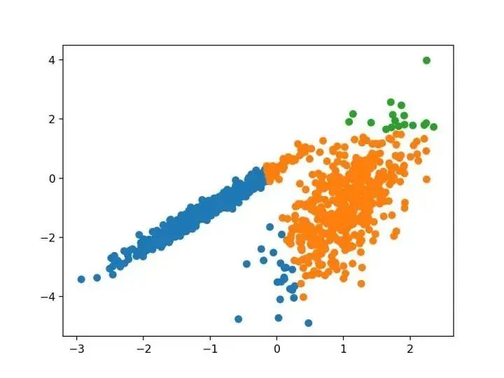
BIRCH 遞增地和動(dòng)態(tài)地群集傳入的多維度量數(shù)據(jù)點(diǎn),以嘗試?yán)每捎觅Y源(即可用內(nèi)存和時(shí)間約束)產(chǎn)生最佳質(zhì)量的聚類。
—源自:《 BIRCH :1996年大型數(shù)據(jù)庫的高效數(shù)據(jù)聚類方法》
# birch聚類
from numpy import unique
from numpy import where
from sklearn.datasets import make_classification
from sklearn.cluster import Birch
from matplotlib import pyplot
# 定義數(shù)據(jù)集
X, _ = make_classification(n_samples=1000, n_features=2, n_informative=2, n_redundant=0, n_clusters_per_class=1, random_state=4)
# 定義模型
model = Birch(threshold=0.01, n_clusters=2)
# 適配模型
model.fit(X)
# 為每個(gè)示例分配一個(gè)集群
yhat = model.predict(X)
# 檢索唯一群集
clusters = unique(yhat)
# 為每個(gè)群集的樣本創(chuàng)建散點(diǎn)圖
for cluster in clusters:
# 獲取此群集的示例的行索引
row_ix = where(yhat == cluster)
# 創(chuàng)建這些樣本的散布
pyplot.scatter(X[row_ix, 0], X[row_ix, 1])
# 繪制散點(diǎn)圖
pyplot.show()

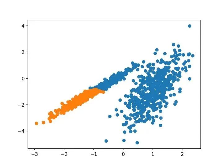
…我們提出了新的聚類算法 DBSCAN 依賴于基于密度的概念的集群設(shè)計(jì),以發(fā)現(xiàn)任意形狀的集群。DBSCAN 只需要一個(gè)輸入?yún)?shù),并支持用戶為其確定適當(dāng)?shù)闹?br style="display: inline;">-源自:《基于密度的噪聲大空間數(shù)據(jù)庫聚類發(fā)現(xiàn)算法》,1996
# dbscan 聚類
from numpy import unique
from numpy import where
from sklearn.datasets import make_classification
from sklearn.cluster import DBSCAN
from matplotlib import pyplot
# 定義數(shù)據(jù)集
X, _ = make_classification(n_samples=1000, n_features=2, n_informative=2, n_redundant=0, n_clusters_per_class=1, random_state=4)
# 定義模型
model = DBSCAN(eps=0.30, min_samples=9)
# 模型擬合與聚類預(yù)測(cè)
yhat = model.fit_predict(X)
# 檢索唯一群集
clusters = unique(yhat)
# 為每個(gè)群集的樣本創(chuàng)建散點(diǎn)圖
for cluster in clusters:
# 獲取此群集的示例的行索引
row_ix = where(yhat == cluster)
# 創(chuàng)建這些樣本的散布
pyplot.scatter(X[row_ix, 0], X[row_ix, 1])
# 繪制散點(diǎn)圖
pyplot.show()
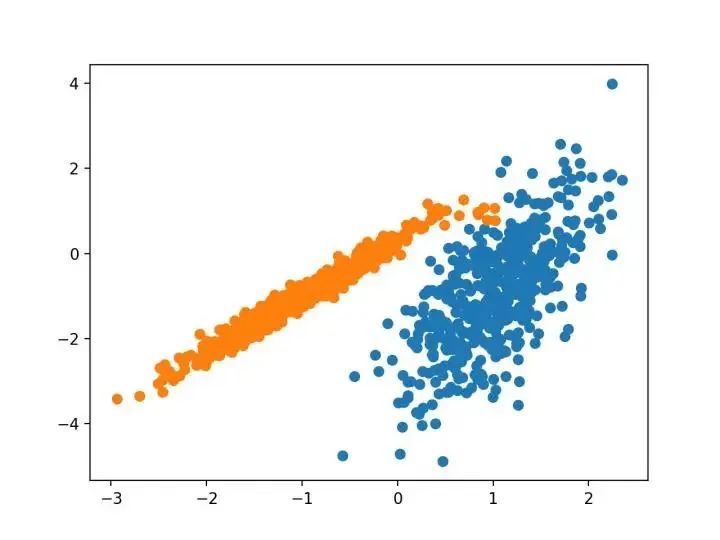
本文的主要目的是描述一種基于樣本將 N 維種群劃分為 k 個(gè)集合的過程。這個(gè)叫做“ K-均值”的過程似乎給出了在類內(nèi)方差意義上相當(dāng)有效的分區(qū)。
-源自:《關(guān)于多元觀測(cè)的分類和分析的一些方法》1967年。
# k-means 聚類
from numpy import unique
from numpy import where
from sklearn.datasets import make_classification
from sklearn.cluster import KMeans
from matplotlib import pyplot
# 定義數(shù)據(jù)集
X, _ = make_classification(n_samples=1000, n_features=2, n_informative=2, n_redundant=0, n_clusters_per_class=1, random_state=4)
# 定義模型
model = KMeans(n_clusters=2)
# 模型擬合
model.fit(X)
# 為每個(gè)示例分配一個(gè)集群
yhat = model.predict(X)
# 檢索唯一群集
clusters = unique(yhat)
# 為每個(gè)群集的樣本創(chuàng)建散點(diǎn)圖
for cluster in clusters:
# 獲取此群集的示例的行索引
row_ix = where(yhat == cluster)
# 創(chuàng)建這些樣本的散布
pyplot.scatter(X[row_ix, 0], X[row_ix, 1])
# 繪制散點(diǎn)圖
pyplot.show()
...我們建議使用 k-均值聚類的迷你批量?jī)?yōu)化。與經(jīng)典批處理算法相比,這降低了計(jì)算成本的數(shù)量級(jí),同時(shí)提供了比在線隨機(jī)梯度下降更好的解決方案。
—源自:《Web-Scale K-均值聚類》2010
# mini-batch k均值聚類
from numpy import unique
from numpy import where
from sklearn.datasets import make_classification
from sklearn.cluster import MiniBatchKMeans
from matplotlib import pyplot
# 定義數(shù)據(jù)集
X, _ = make_classification(n_samples=1000, n_features=2, n_informative=2, n_redundant=0, n_clusters_per_class=1, random_state=4)
# 定義模型
model = MiniBatchKMeans(n_clusters=2)
# 模型擬合
model.fit(X)
# 為每個(gè)示例分配一個(gè)集群
yhat = model.predict(X)
# 檢索唯一群集
clusters = unique(yhat)
# 為每個(gè)群集的樣本創(chuàng)建散點(diǎn)圖
for cluster in clusters:
# 獲取此群集的示例的行索引
row_ix = where(yhat == cluster)
# 創(chuàng)建這些樣本的散布
pyplot.scatter(X[row_ix, 0], X[row_ix, 1])
# 繪制散點(diǎn)圖
pyplot.show()
對(duì)離散數(shù)據(jù)證明了遞推平均移位程序收斂到最接近駐點(diǎn)的基礎(chǔ)密度函數(shù),從而證明了它在檢測(cè)密度模式中的應(yīng)用。
—源自:《Mean Shift :面向特征空間分析的穩(wěn)健方法》,2002
# 均值漂移聚類
from numpy import unique
from numpy import where
from sklearn.datasets import make_classification
from sklearn.cluster import MeanShift
from matplotlib import pyplot
# 定義數(shù)據(jù)集
X, _ = make_classification(n_samples=1000, n_features=2, n_informative=2, n_redundant=0, n_clusters_per_class=1, random_state=4)
# 定義模型
model = MeanShift()
# 模型擬合與聚類預(yù)測(cè)
yhat = model.fit_predict(X)
# 檢索唯一群集
clusters = unique(yhat)
# 為每個(gè)群集的樣本創(chuàng)建散點(diǎn)圖
for cluster in clusters:
# 獲取此群集的示例的行索引
row_ix = where(yhat == cluster)
# 創(chuàng)建這些樣本的散布
pyplot.scatter(X[row_ix, 0], X[row_ix, 1])
# 繪制散點(diǎn)圖
pyplot.show()
我們?yōu)榫垲惙治鲆肓艘环N新的算法,它不會(huì)顯式地生成一個(gè)數(shù)據(jù)集的聚類;而是創(chuàng)建表示其基于密度的聚類結(jié)構(gòu)的數(shù)據(jù)庫的增強(qiáng)排序。此群集排序包含相當(dāng)于密度聚類的信息,該信息對(duì)應(yīng)于范圍廣泛的參數(shù)設(shè)置。
—源自:《OPTICS :排序點(diǎn)以標(biāo)識(shí)聚類結(jié)構(gòu)》,1999
# optics聚類
from numpy import unique
from numpy import where
from sklearn.datasets import make_classification
from sklearn.cluster import OPTICS
from matplotlib import pyplot
# 定義數(shù)據(jù)集
X, _ = make_classification(n_samples=1000, n_features=2, n_informative=2, n_redundant=0, n_clusters_per_class=1, random_state=4)
# 定義模型
model = OPTICS(eps=0.8, min_samples=10)
# 模型擬合與聚類預(yù)測(cè)
yhat = model.fit_predict(X)
# 檢索唯一群集
clusters = unique(yhat)
# 為每個(gè)群集的樣本創(chuàng)建散點(diǎn)圖
for cluster in clusters:
# 獲取此群集的示例的行索引
row_ix = where(yhat == cluster)
# 創(chuàng)建這些樣本的散布
pyplot.scatter(X[row_ix, 0], X[row_ix, 1])
# 繪制散點(diǎn)圖
pyplot.show()
最近在許多領(lǐng)域出現(xiàn)的一個(gè)有希望的替代方案是使用聚類的光譜方法。這里,使用從點(diǎn)之間的距離導(dǎo)出的矩陣的頂部特征向量。
—源自:《關(guān)于光譜聚類:分析和算法》,2002年
# spectral clustering
from numpy import unique
from numpy import where
from sklearn.datasets import make_classification
from sklearn.cluster import SpectralClustering
from matplotlib import pyplot
# 定義數(shù)據(jù)集
X, _ = make_classification(n_samples=1000, n_features=2, n_informative=2, n_redundant=0, n_clusters_per_class=1, random_state=4)
# 定義模型
model = SpectralClustering(n_clusters=2)
# 模型擬合與聚類預(yù)測(cè)
yhat = model.fit_predict(X)
# 檢索唯一群集
clusters = unique(yhat)
# 為每個(gè)群集的樣本創(chuàng)建散點(diǎn)圖
for cluster in clusters:
# 獲取此群集的示例的行索引
row_ix = where(yhat == cluster)
# 創(chuàng)建這些樣本的散布
pyplot.scatter(X[row_ix, 0], X[row_ix, 1])
# 繪制散點(diǎn)圖
pyplot.show()
# 高斯混合模型
from numpy import unique
from numpy import where
from sklearn.datasets import make_classification
from sklearn.mixture import GaussianMixture
from matplotlib import pyplot
# 定義數(shù)據(jù)集
X, _ = make_classification(n_samples=1000, n_features=2, n_informative=2, n_redundant=0, n_clusters_per_class=1, random_state=4)
# 定義模型
model = GaussianMixture(n_components=2)
# 模型擬合
model.fit(X)
# 為每個(gè)示例分配一個(gè)集群
yhat = model.predict(X)
# 檢索唯一群集
clusters = unique(yhat)
# 為每個(gè)群集的樣本創(chuàng)建散點(diǎn)圖
for cluster in clusters:
# 獲取此群集的示例的行索引
row_ix = where(yhat == cluster)
# 創(chuàng)建這些樣本的散布
pyplot.scatter(X[row_ix, 0], X[row_ix, 1])
# 繪制散點(diǎn)圖
pyplot.show()

在本教程中,您發(fā)現(xiàn)了如何在 python 中安裝和使用頂級(jí)聚類算法。具體來說,你學(xué)到了:
聚類是在特征空間輸入數(shù)據(jù)中發(fā)現(xiàn)自然組的無監(jiān)督問題。
有許多不同的聚類算法,對(duì)于所有數(shù)據(jù)集沒有單一的最佳方法。
在 scikit-learn 機(jī)器學(xué)習(xí)庫的 Python 中如何實(shí)現(xiàn)、適合和使用頂級(jí)聚類算法。
加入知識(shí)星球【我們談?wù)摂?shù)據(jù)科學(xué)】
500+小伙伴一起學(xué)習(xí)!
·?推薦閱讀?·
在jupyter中實(shí)現(xiàn)實(shí)時(shí)協(xié)同是一種什么體驗(yàn)