
【深度學(xué)習(xí)】RetinaNet 代碼完全解析
本文就是大名鼎鼎的focalloss中提出的網(wǎng)絡(luò),其基本結(jié)構(gòu)backbone+fpn+head也是目前目標(biāo)檢測算法的標(biāo)準(zhǔn)結(jié)構(gòu)。RetinaNet憑借結(jié)構(gòu)精簡,清晰明了、可擴(kuò)展性強(qiáng)、效果優(yōu)秀,成為了很多算法的baseline。本文不去過多從理論分析focalloss的機(jī)制,從代碼角度解析RetinaNet的實現(xiàn)過程,尤其是anchor生成與匹配、loss計算過程。
論文鏈接:
參考代碼鏈接:
網(wǎng)絡(luò)結(jié)構(gòu)
網(wǎng)絡(luò)結(jié)構(gòu)非常清晰明了,使用的組件都是標(biāo)準(zhǔn)公認(rèn)的,并且容易替換掉的。在這里,你不會看到SSD沒有特征融合的多尺度,你也不會看到只有yolo才用的darknet。預(yù)測輸出就是類別+位置,也是目標(biāo)檢測任務(wù)面臨的本質(zhì)。
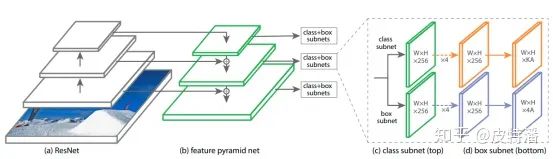
FPN
這部分無需過多介紹,就是融合不同尺度的特征,融合的方式一般是element-wise相加。當(dāng)遇到尺度不一致時,利用卷積+上采樣操作來處理。為了清晰理解,給出實例:
一般backbone會提取4層特征,尺度分別是,假設(shè)batch為1:
c2:1*64*W/4*H/4
c3:1*128*W/8*H/8
c4:1*256*W/16*H/16
c5:1*512*W/32*H/32:
這里只需要后三層特征;假設(shè)輸入數(shù)據(jù)為[1,3,320,320],F(xiàn)PN輸出的特征維度分別為:
torch.Size([1, 256, 40, 40])
torch.Size([1, 256, 20, 20])
torch.Size([1, 256, 10, 10])
torch.Size([1, 256, 5, 5])
torch.Size([1, 256, 3, 3])
當(dāng)然FPN是非常容易定制的組件,當(dāng)你的場景不需要太多尺度的話,可以刪減輸出分支。
Head
Fpn輸出的分支,每一個都會進(jìn)行分類和回歸操作
分類輸出
每層特征經(jīng)過4次卷積+relu操作,然后再通過head 卷積
self.output = nn.Conv2d(feature_size, num_anchors * num_classes, kernel_size=3, padding=1)
self.output_act = nn.Sigmoid()
輸出最終預(yù)測輸出,尺度是
torch.Size([1, 14400, 80])
torch.Size([1, 3600, 80])
torch.Size([1, 900, 80])
torch.Size([1, 225, 80])
torch.Size([1, 81, 80])
其中14400 = 40*40*9,9為anchor個數(shù),最后在把所有結(jié)果拼接在一起[1,19206,80]的tensor。可以理解為每一個特征圖位置預(yù)測9個anchor,每個anchor具有80個類別。拼接操作為了和anchor的形式統(tǒng)一起來,方便計算loss和前向預(yù)測。注意,這里的激活函數(shù)使用的是sigmoid(),如果你想使用softmax()輸出,那么就需要增加一個類別。不過論文證明了Sigmoid()效果要優(yōu)于softmax().
回歸輸出
和分類頭類似,同樣是4層卷積+relu()操作,最后是輸出卷積。由于是回歸問題,所以沒有進(jìn)行激活操作。
self.output = nn.Conv2d(feature_size, num_anchors * 4, kernel_size=3, padding=1)尺度變化為:
torch.Size([1, 14400, 4])
torch.Size([1, 3600, 4])
torch.Size([1, 900, 4])
torch.Size([1, 225, 4])
torch.Size([1, 81, 4])
最后在把所有結(jié)果拼接在一起[1,19206,4],4代表預(yù)測box的中心點+寬高。
Anchor生成
大的特征圖預(yù)測小的物體,小的特征圖預(yù)測大的物體,fpn有5個輸出,所以會有5中尺度的anchor,每種尺度又分為9中寬高比。
首先定義特征圖的level:
self.pyramid_levels = [3, 4, 5, 6, 7]獲取對應(yīng)stride為:
self.strides = [2 ** x for x in self.pyramid_levels]
# [8,16,32,64,128]
獲取每一層上的base size:
self.sizes = [2 ** (x + 2) for x in self.pyramid_levels]
# [32,64,128,256,512]
將3種框高比和3個scale進(jìn)行搭配,獲取9個anchor:
ratios = np.array([0.5, 1, 2])
scales = np.array([2 ** 0, 2 ** (1.0 / 3.0), 2 ** (2.0 / 3.0)])=[1,1.26,1.587]
首先計算大小:
anchors[:, 2:] = base_size * np.tile(scales, (2, len(ratios))).T獲取初步的anchor的寬高 (舉例,最小的輸出層):
[[ 0.          0.         32.         32.        ]
 [ 0.          0.         40.3174736  40.3174736 ]
 [ 0.          0.         50.79683366 50.79683366]
 [ 0.          0.         32.         32.        ]
 [ 0.          0.         40.3174736  40.3174736 ]
 [ 0.          0.         50.79683366 50.79683366]
 [ 0.          0.         32.         32.        ]
 [ 0.          0.         40.3174736  40.3174736 ]
 [ 0.          0.         50.79683366 50.79683366]]
獲取每一種尺度的面積:
[1024. 1625. 2580. 1024. 1625. 2580. 1024. 1625. 2580.]然后按照寬高比生成anchor:
[[ 0.          0.         45.254834   22.627417  ]
 [ 0.          0.         57.01751796 28.50875898]
 [ 0.          0.         71.83757109 35.91878555]
 [ 0.          0.         32.         32.        ]
 [ 0.          0.         40.3174736  40.3174736 ]
 [ 0.          0.         50.79683366 50.79683366]
 [ 0.          0.         22.627417   45.254834  ]
 [ 0.          0.         28.50875898 57.01751796]
 [ 0.          0.         35.91878555 71.83757109]]
最后轉(zhuǎn)化為xyxy的形式:
[[-22.627417   -11.3137085   22.627417    11.3137085 ]
 [-28.50875898 -14.25437949  28.50875898  14.25437949]
 [-35.91878555 -17.95939277  35.91878555  17.95939277]
 [-16.         -16.          16.          16.        ]
 [-20.1587368  -20.1587368   20.1587368   20.1587368 ]
 [-25.39841683 -25.39841683  25.39841683  25.39841683]
 [-11.3137085  -22.627417    11.3137085   22.627417  ]
 [-14.25437949 -28.50875898  14.25437949  28.50875898]
 [-17.95939277 -35.91878555  17.95939277  35.91878555]]
因此獲取了其中一層的base anchor,這組anchor是特征圖上位置(0,0)的特征圖片,只需要復(fù)制+平移到其他位置,就可以獲取整張?zhí)卣鲌D上所有的anchor。其他尺度的特征圖做法類似最后將所有特征圖上的anchor拼接起來,size同樣為為[1,19206,4]
anchor編碼
代碼沒有將anchor編碼拆分成一個獨立的模塊,
首先gt box轉(zhuǎn)化成中心點和寬高的形式:
gt_widths  = assigned_annotations[:, 2] - assigned_annotations[:, 0]
gt_heights = assigned_annotations[:, 3] - assigned_annotations[:, 1]
gt_ctr_x   = assigned_annotations[:, 0] + 0.5 * gt_widths
gt_ctr_y   = assigned_annotations[:, 1] + 0.5 * gt_heights
同理anchor也轉(zhuǎn)換成中心點和寬高的形式:
anchor_widths  = anchor[:, 2] - anchor[:, 0]
anchor_heights = anchor[:, 3] - anchor[:, 1]
anchor_ctr_x   = anchor[:, 0] + 0.5 * anchor_widths
anchor_ctr_y   = anchor[:, 1] + 0.5 * anchor_heights
計算二者的相對值
targets_dx = (gt_ctr_x - anchor_ctr_x_pi) / anchor_widths_pi
targets_dy = (gt_ctr_y - anchor_ctr_y_pi) / anchor_heights_pi
targets_dw = torch.log(gt_widths / anchor_widths_pi)
targets_dh = torch.log(gt_heights / anchor_heights_pi)
當(dāng)然我們的目標(biāo)就是網(wǎng)絡(luò)預(yù)測值和這四個相對值相等。
anchor分配
這部分主要是根據(jù)iou的大小劃分正負(fù)樣本,既挑出那些負(fù)責(zé)預(yù)測gt的anchor。分配的策略非常簡單,就是iou策略。
需要求iou:
IoU_max, IoU_argmax = torch.max(IoU, dim=1) # num_anchors x 1正樣本:和gt的iou大于0.5的ancho樣本
負(fù)樣本:和gt的iou小于0.4的anchor
忽略樣本:其他anchor
問題:沒有像yolo系列一樣,如果沒有大于0.5的anchor預(yù)測,至少會分配一個iou最大的anchor。因為retinanet認(rèn)為coco數(shù)據(jù)集按照此策略,匹配不到的情況非常少。
loss計算
focal loss 請參考:

當(dāng)圖片沒有目標(biāo)時,只計算分類loss,不計算box位置loss,所有anchor都是負(fù)樣本:
alpha_factor = torch.ones(classification.shape) * alpha

alpha_factor = 1. - alpha_factor
focal_weight = classification
focal_weight = alpha_factor * torch.pow(focal_weight, gamma)

bce = -(torch.log(1.0 - classification))

cls_loss = focal_weight * bce
classification_losses.append(cls_loss.sum())
# 回歸loss為0
regression_losses.append(torch.tensor(0).float())
分類loss:
# 注意,這里是利用sigmoid輸出,可以直接使用alpha和1-alpha。每一個分支都在做目標(biāo)和背景的二分類
alpha_factor = torch.where(torch.eq(targets, 1.), alpha_factor, 1. - alpha_factor)
focal_weight = torch.where(torch.eq(targets, 1.), 1. - classification, classification)
focal_weight = alpha_factor * torch.pow(focal_weight, gamma)
bce = -(targets * torch.log(classification) + (1.0 - targets) * torch.log(1.0 - classification))
cls_loss = focal_weight * bce
回歸loss:
# 只在正樣本的anchor上計算,abs就是f1 loss
regression_diff = torch.abs(targets - regression[positive_indices, :])
# 進(jìn)行smooth一下,就是smooth l1 loss
regression_loss = torch.where(
                    torch.le(regression_diff, 1.0 / 9.0),
                    0.5 * 9.0 * torch.pow(regression_diff, 2),
                    regression_diff - 0.5 / 9.0)
測試推理
因為測試推理過程一般比較簡單,部分代碼如下:
def forward(self, boxes, deltas):
    widths  = boxes[:, :, 2] - boxes[:, :, 0]
    heights = boxes[:, :, 3] - boxes[:, :, 1]
    ctr_x   = boxes[:, :, 0] + 0.5 * widths
    ctr_y   = boxes[:, :, 1] + 0.5 * heights

    dx = deltas[:, :, 0] * self.std[0] + self.mean[0]
    dy = deltas[:, :, 1] * self.std[1] + self.mean[1]
    dw = deltas[:, :, 2] * self.std[2] + self.mean[2]
    dh = deltas[:, :, 3] * self.std[3] + self.mean[3]
'''其中boxes為anchor,deltas為網(wǎng)絡(luò)回歸的box分支。
注意這里的self.std[0] + self.mean[0]是對輸出的標(biāo)準(zhǔn)化逆向操作,
因為網(wǎng)絡(luò)輸出時的監(jiān)督有標(biāo)準(zhǔn)化操作。使用的均值和方差是固定數(shù)值。
目的是對相對數(shù)值進(jìn)行放大,幫助網(wǎng)絡(luò)回歸'''

    pred_ctr_x = ctr_x + dx * widths
    pred_ctr_y = ctr_y + dy * heights
    pred_w     = torch.exp(dw) * widths
    pred_h     = torch.exp(dh) * heights

    pred_boxes_x1 = pred_ctr_x - 0.5 * pred_w
    pred_boxes_y1 = pred_ctr_y - 0.5 * pred_h
    pred_boxes_x2 = pred_ctr_x + 0.5 * pred_w
    pred_boxes_y2 = pred_ctr_y + 0.5 * pred_h

    pred_boxes = torch.stack([pred_boxes_x1, pred_boxes_y1, pred_boxes_x2, pred_boxes_y2], dim=2)

 return pred_boxes
解碼完成后,獲得真實預(yù)測的box,還要經(jīng)過clipBoxes操作,就是保證所有數(shù)不會超過圖片的尺度范圍。然后對每一個類別進(jìn)行遍歷,獲取類別的score,提取大于一定閾的box,再進(jìn)行nms就可以了。沒啥。
結(jié)語
RetinaNet是一個結(jié)構(gòu)非常清晰的目標(biāo)檢測框架,backbone以及neck的FPN非常容易更換掉,head的定義也非常簡單。又有focal loss的加成,成為了很多算法baseline,例如任意角度的目標(biāo)檢測。本文從代碼層面進(jìn)行剖析,希望和大家一起學(xué)習(xí)。
往期精彩回顧
獲取本站知識星球優(yōu)惠券,復(fù)制鏈接直接打開:
https://t.zsxq.com/qFiUFMV
本站qq群704220115。
加入微信群請掃碼: