黄色天堂,淫交黑料吃瓜AV,日本三级在线观看中文字串,色色一级免费电影,国产无码福利在线,日韩欧美手机在线观看,三级网站播放,国产成人久久视频

最強(qiáng) Python 數(shù)據(jù)可視化庫(kù)，沒有之一！關(guān)注"Python學(xué)習(xí)與數(shù)據(jù)挖掘"

設(shè)為“置頂或星標(biāo)”，第一時(shí)間送達(dá)干貨

資料專欄

李航老師《統(tǒng)計(jì)學(xué)習(xí)方法（第二版）》課件&代碼

【視頻+PPT】李宏毅老師機(jī)器學(xué)習(xí)40講

來自數(shù)據(jù)STUDIO

大家好，我是城哥。

今天給大家分享一篇模型超參調(diào)優(yōu)的可視化方法：Hyperopt+plotly

本文將演示如何創(chuàng)建超參數(shù)設(shè)置的有效交互式可視化，使我們能夠了解在超參數(shù)優(yōu)化期間嘗試的超參數(shù)設(shè)置之間的關(guān)系。本文的第 1 部分將使用 hyperopt 設(shè)置一個(gè)簡(jiǎn)單的超參數(shù)優(yōu)化示例。在第 2 部分中，我們將展示如何使用Plotly創(chuàng)建由第 1 部分中的超參數(shù)優(yōu)化生成的數(shù)據(jù)的交互式可視化。

至今，很多大佬對(duì)“超參數(shù)優(yōu)化”算法進(jìn)行了大量研究，這些算法在進(jìn)行少量配置后會(huì)自動(dòng)搜索最佳超參數(shù)集。這些算法可以通過各種 Python 包實(shí)現(xiàn)。例如hyperopt就是其中一個(gè)廣泛使用的超參數(shù)優(yōu)化框架包，它允許數(shù)據(jù)科學(xué)家通過定義目標(biāo)函數(shù)和聲明搜索空間來利用幾種強(qiáng)大的算法進(jìn)行超參數(shù)優(yōu)化。

然而，依靠這些工具可以將超參數(shù)選擇變成一個(gè)“黑匣子”，這也導(dǎo)致了很難解釋為什么一組特定的超參數(shù)最適合一個(gè)特定問題的特定模型。克服這些算法的“黑匣子”性質(zhì)的一種方法，是可視化在超參數(shù)優(yōu)化期間嘗試過的超參數(shù)設(shè)置的歷史，以幫助識(shí)別運(yùn)行良好的超參數(shù)設(shè)置的潛在趨勢(shì)。

寫在前面

這篇文章假設(shè)讀者熟悉超參數(shù)優(yōu)化的概念。此外，盡管我們將創(chuàng)建一個(gè)示例超參數(shù)優(yōu)化來生成可視化所需要的數(shù)據(jù)，但我們不會(huì)詳細(xì)介紹此優(yōu)化，因?yàn)楸疚牡哪康牟皇浅蔀橛嘘P(guān) hyperopt 的教程；這里有個(gè)不錯(cuò)的hyperopt 文檔英文教程^[1]。

為簡(jiǎn)潔起見，代碼示例將假設(shè)所有必要的導(dǎo)入都已運(yùn)行。作為參考，這里是代碼示例所需的完整導(dǎo)入集：

from?functools?import?partial
from?pprint?import?pprint

import?numpy?as?np
import?pandas?as?pd

from?hyperopt?import?fmin,?hp,?space_eval,?tpe,?STATUS_OK,?Trials
from?hyperopt.pyll?import?scope,?stochastic
from?plotly?import?express?as?px
from?plotly?import?graph_objects?as?go
from?plotly?import?offline?as?pyo
from?sklearn.datasets?import?load_boston
from?sklearn.ensemble?import?GradientBoostingRegressor,?RandomForestRegressor
from?sklearn.metrics?import?make_scorer,?mean_squared_error
from?sklearn.model_selection?import?cross_val_score,?KFold
from?sklearn.utils?import?check_random_state

pyo.init_notebook_mode()

使用 hyperopt 超參數(shù)優(yōu)化示例

在我們使用 Plotly 進(jìn)行可視化之前，我們需要從 hyperopt 生成一些超參數(shù)優(yōu)化數(shù)據(jù)供我們可視化。我們需要遵循四個(gè)關(guān)鍵步驟來使用 hyperopt 設(shè)置超參數(shù)優(yōu)化：

選擇和加載數(shù)據(jù)集
聲明超參數(shù)搜索空間
定義目標(biāo)函數(shù)
運(yùn)行超參數(shù)優(yōu)化

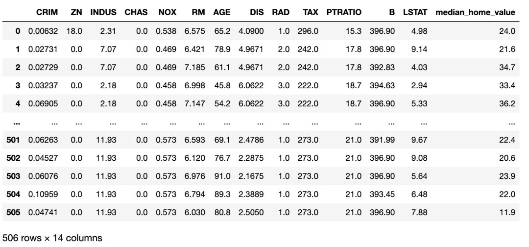
我們將提供每個(gè)步驟的簡(jiǎn)要描述以及示例代碼，但我們不會(huì)詳細(xì)說明具體選擇的合理性，因?yàn)檫@種超參數(shù)優(yōu)化的目標(biāo)只是為我們生成可視化數(shù)據(jù)。

選擇和加載數(shù)據(jù)集

我們將使用UCI^[2]波士頓數(shù)據(jù)集作為我們的超參數(shù)優(yōu)化的示例數(shù)據(jù)集。UCI 波士頓數(shù)據(jù)集的特征是各種社區(qū)特征，目標(biāo)是該社區(qū)房屋的中值。Scikit-learn 提供了一個(gè)方便的包裝函數(shù)，名為load_boston。我們將使用此函數(shù)將數(shù)據(jù)集加載到 Pandas 數(shù)據(jù)框中，如下所示：

MEDIAN_HOME_VALUE?=?"median_home_value"

#?使用?sklearn?的輔助函數(shù)加載波士頓數(shù)據(jù)集
boston_dataset?=?load_boston()
#?將數(shù)據(jù)轉(zhuǎn)換為?Pandas?數(shù)據(jù)框
data?=?np.concatenate(
????[boston_dataset["data"],?boston_dataset["target"][...,?np.newaxis]],
????axis=1,
)
features,?target?=?boston_dataset["feature_names"],?MEDIAN_HOME_VALUE
columns?=?np.concatenate([features,?[target]])
boston_dataset_df?=?pd.DataFrame(data,?columns=columns)
boston_dataset_df

定義超參數(shù)搜索空間

由于該數(shù)據(jù)集的目標(biāo)是連續(xù)的，我們將要比較幾個(gè)不同的回歸模型。我們將設(shè)置超參數(shù)優(yōu)化來比較兩種類型的模型：隨機(jī)森林回歸器和梯度提升回歸器（可以閱讀文檔戳??集成算法｜隨機(jī)森林回歸模型）。隨機(jī)森林回歸器將允許 hyperopt 調(diào)整樹的數(shù)量和每棵樹的最大深度。除了樹的數(shù)量和每棵樹的最大深度之外，梯度提升回歸器將允許 hyperopt 調(diào)整學(xué)習(xí)率。以下字典以 hyperopt 預(yù)期的格式聲明此超參數(shù)搜索空間：

#?定義常量字符串，我們將在下面的“search space”字典中用作鍵。
#?注意，我在整個(gè)過程中使用的約定是，
#?用一個(gè)匹配該字符串的變量來表示字符串中的字符，只是變量中的字符是大寫的。
#?這種約定允許我們?cè)诖a中遇到這些變量時(shí)很容易解釋它們的含義。
#?例如，我們知道變量' MODEL '包含字符串" MODEL "。
#?用變量表示字符串的這種模式允許我在代碼中重復(fù)使用同一個(gè)字符串時(shí)避免鍵入錯(cuò)誤，
#?因?yàn)樵谧兞棵墟I入錯(cuò)誤將被檢查器捕獲為錯(cuò)誤。

GRADIENT_BOOSTING_REGRESSOR?=?"gradient_boosting_regressor"
KWARGS?=?"kwargs"
LEARNING_RATE?=?"learning_rate"
LINEAR_REGRESSION?=?"linear_regression"
MAX_DEPTH?=?"max_depth"
MODEL?=?"model"
MODEL_CHOICE?=?"model_choice"
NORMALIZE?=?"normalize"
N_ESTIMATORS?=?"n_estimators"
RANDOM_FOREST_REGRESSOR?=?"random_forest_regressor"
RANDOM_STATE?=?"random_state"

#?聲明隨機(jī)森林回歸模型的搜索空間。
random_forest_regressor?=?{
????MODEL:?RANDOM_FOREST_REGRESSOR,
???#?我將模型參數(shù)定義為一個(gè)單獨(dú)的字典，以便我們可以將參數(shù)輸入
???#?帶有字典解包的模型的`__init__`。參見?`sample_to_model`?函數(shù)
???#?與目標(biāo)函數(shù)一起定義以查看此操作
????KWARGS:?{
????????N_ESTIMATORS:?scope.int(
????????????hp.quniform(f"{RANDOM_FOREST_REGRESSOR}__{N_ESTIMATORS}",?50,?150,?1)
????????),
????????MAX_DEPTH:?scope.int(
????????????hp.quniform(f"{RANDOM_FOREST_REGRESSOR}__{MAX_DEPTH}",?2,?12,?1)
????????),
????????RANDOM_STATE:?0,
????},
}

#?聲明梯度提升回歸模型的搜索空間，
#?結(jié)構(gòu)與隨機(jī)森林回歸搜索空間相同。
gradient_boosting_regressor?=?{
????MODEL:?GRADIENT_BOOSTING_REGRESSOR,
????KWARGS:?{
????????LEARNING_RATE:?scope.float(
????????????hp.uniform(f"{GRADIENT_BOOSTING_REGRESSOR}__{LEARNING_RATE}",?0.01,?0.15,)
????????),??#?lower?learning?rate
????????N_ESTIMATORS:?scope.int(
????????????hp.quniform(f"{GRADIENT_BOOSTING_REGRESSOR}__{N_ESTIMATORS}",?50,?150,?1)
????????),
????????MAX_DEPTH:?scope.int(
????????????hp.quniform(f"{GRADIENT_BOOSTING_REGRESSOR}__{MAX_DEPTH}",?2,?12,?1)
????????),
????????RANDOM_STATE:?0,
????},
}

#?將兩個(gè)模型搜索空間與兩個(gè)模型之間的頂級(jí)“choice”結(jié)合起來，得到最終的搜索空間。
space?=?{
????MODEL_CHOICE:?hp.choice(
????????MODEL_CHOICE,?[random_forest_regressor,?gradient_boosting_regressor,],
????)
}

定義目標(biāo)函數(shù)

對(duì)于目標(biāo)函數(shù)，我們將通過十折交叉驗(yàn)證計(jì)算數(shù)據(jù)集每個(gè)實(shí)例的均方誤差。我們將打印折疊的平均均方誤差作為損失。下面的代碼定義了這個(gè)目標(biāo)：

#?定義幾個(gè)額外的變量來表示字符串。注意，這段代碼期望我們能夠
#?訪問之前在"search space"代碼片段中定義的所有變量。
LOSS?=?"loss"
STATUS?=?"status"

#?從字符串名稱映射到模型類定義對(duì)象，我們將使用該對(duì)象
#?從hyperopt搜索空間生成的樣本創(chuàng)建模型的初始化版本。
MODELS?=?{
????GRADIENT_BOOSTING_REGRESSOR:?GradientBoostingRegressor,
????RANDOM_FOREST_REGRESSOR:?RandomForestRegressor,
}
#?創(chuàng)建一個(gè)我們將在目標(biāo)中使用的評(píng)分函數(shù)
mse_scorer?=?make_scorer(mean_squared_error)


#?從hyperopt生成的示例轉(zhuǎn)換為初始化模型的輔助函數(shù)。
#?注意，因?yàn)槲覀冊(cè)谒阉骺臻g聲明中將模型類型和模型關(guān)鍵字-參數(shù)分割成單獨(dú)的鍵-值對(duì)，#?所以我們能夠使用字典解包來創(chuàng)建模型的初始化版本。
def?sample_to_model(sample):
????kwargs?=?sample[MODEL_CHOICE][KWARGS]
????return?MODELS[sample[MODEL_CHOICE][MODEL]](**kwargs?"sample[MODEL_CHOICE][MODEL]")


#?定義hyperopt的目標(biāo)函數(shù)。我們將使用?`functools.partial`?修復(fù)`dataset`, `features`, 和?`target`?參數(shù)。
#?來創(chuàng)建這個(gè)函數(shù)的那個(gè)版本,?并將其作為參數(shù)提供給?`fmin`
def?objective(sample,?dataset_df,?features,?target):
????model?=?sample_to_model(sample)
????rng?=?check_random_state(0)
#?處理隨機(jī)洗牌時(shí)創(chuàng)建折疊。在現(xiàn)實(shí)中，
#?我們可能需要比上述生成的固定“RandomState”實(shí)例更好的策略來管理隨機(jī)性。
????cv?=?KFold(n_splits=10,?random_state=rng,?shuffle=True)
#?計(jì)算每一次的平均均方誤差。由于`n_splits`?是10，`mse`?將是一個(gè)大小為10的數(shù)組，
#?每個(gè)元素表示一次折疊的平均平均平方誤差。
????mse?=?cross_val_score(
????????model,
????????dataset_df.loc[:,?features],
????????dataset_df.loc[:,?target],
????????scoring=mse_scorer,
????????cv=cv,
????)
????#?返回所有折疊的均方誤差的平均值。
????return?{LOSS:?np.mean(mse),?STATUS:?STATUS_OK}

運(yùn)行超參數(shù)優(yōu)化

我們將通過調(diào)用fmin函數(shù)運(yùn)行一千次試驗(yàn)的超參數(shù)優(yōu)化。重要的是，我們將提供一個(gè)Trials對(duì)象的實(shí)例，hyperopt 將在其中記錄超參數(shù)優(yōu)化的每次迭代的超參數(shù)設(shè)置。我們將從這個(gè)Trials實(shí)例中提取可視化數(shù)據(jù)。運(yùn)行以下代碼執(zhí)行超參數(shù)優(yōu)化：

#?我們自定義的目標(biāo)函數(shù)是通用的數(shù)據(jù)集,
#?我們需要使用`partial`?從`functools`?模塊來"fix"這個(gè)`dataset_df`,?`features`,?和?`target`?的參數(shù)值,
#?希望在這個(gè)例子中,我們有一個(gè)目標(biāo)函數(shù)只接受一個(gè)參數(shù)假設(shè)的“hyperopt”界面。

boston_objective?=?partial(
????objective,?dataset_df=boston_dataset_df,?features=features,?target=MEDIAN_HOME_VALUE
)
#?`hyperopt`?跟蹤這個(gè)`Trials`對(duì)象的每次迭代的結(jié)果。
#?我們將從這個(gè)對(duì)象中收集用于可視化的數(shù)據(jù)。
trials?=?Trials()
rng?=?check_random_state(0)??#?reproducibility!
#?`fmin`搜索“minimize”我們的對(duì)象的超參數(shù)，均方誤差，并返回超參數(shù)的“best”集。
best?=?fmin(boston_objective,?space,?tpe.suggest,?1000,?trials=trials,?rstate=rng)

超參數(shù)優(yōu)化可視化

Hyperopt 記錄在超參數(shù)優(yōu)化期間嘗試的超參數(shù)設(shè)置的歷史記錄在我們作為參數(shù)提供給調(diào)用 fmin 的 Trials 對(duì)象的實(shí)例中。優(yōu)化完成后，我們可以檢查trials變量以查看 hyperopt 為前五個(gè)試驗(yàn)選擇了哪些設(shè)置，如下所示：

pprint([t?for?t?in?trials][:5])

[{'book_time': datetime.datetime(2020, 11, 4, 0, 51, 42, 199000),
  'exp_key': None,
  'misc': {'cmd': ('domain_attachment', 'FMinIter_Domain'),
           'idxs': {'gradient_boosting_regressor__learning_rate': [],
                    'gradient_boosting_regressor__max_depth': [],
                    'gradient_boosting_regressor__n_estimators': [],
                    'model_choice': [0],
                    'random_forest_regressor__max_depth': [0],
                    'random_forest_regressor__n_estimators': [0]},
           'tid': 0,
           'vals': {'gradient_boosting_regressor__learning_rate': [],
                    'gradient_boosting_regressor__max_depth': [],
                    'gradient_boosting_regressor__n_estimators': [],
                    'model_choice': [0],
                    'random_forest_regressor__max_depth': [5.0],
                    'random_forest_regressor__n_estimators': [90.0]},
           'workdir': None},
  'owner': None,
  'refresh_time': datetime.datetime(2020, 11, 4, 0, 51, 46, 83000),
  'result': {'loss': 16.359897953574603, 'status': 'ok'},
  'spec': None,
  'state': 2,
  'tid': 0,
  'version': 0},
 {'book_time': datetime.datetime(2020, 11, 4, 0, 51, 46, 92000),
  'exp_key': None,
  'misc': {'cmd': ('domain_attachment', 'FMinIter_Domain'),
           'idxs': {'gradient_boosting_regressor__learning_rate': [1],
                    'gradient_boosting_regressor__max_depth': [1],
                    'gradient_boosting_regressor__n_estimators': [1],
                    'model_choice': [1],
                    'random_forest_regressor__max_depth': [],
                    'random_forest_regressor__n_estimators': []},
           'tid': 1,
           'vals': {'gradient_boosting_regressor__learning_rate': [0.03819110609989756],
                    'gradient_boosting_regressor__max_depth': [8.0],
                    'gradient_boosting_regressor__n_estimators': [137.0],
                    'model_choice': [1],
                    'random_forest_regressor__max_depth': [],
                    'random_forest_regressor__n_estimators': []},
           'workdir': None},
  'owner': None,
  'refresh_time': datetime.datetime(2020, 11, 4, 0, 51, 52, 70000),
  'result': {'loss': 18.045981512632412, 'status': 'ok'},
  'spec': None,
  'state': 2,
  'tid': 1,
  'version': 0},
 {'book_time': datetime.datetime(2020, 11, 4, 0, 51, 52, 81000),
  'exp_key': None,
  'misc': {'cmd': ('domain_attachment', 'FMinIter_Domain'),
           'idxs': {'gradient_boosting_regressor__learning_rate': [2],
                    'gradient_boosting_regressor__max_depth': [2],
                    'gradient_boosting_regressor__n_estimators': [2],
                    'model_choice': [2],
                    'random_forest_regressor__max_depth': [],
                    'random_forest_regressor__n_estimators': []},
           'tid': 2,
           'vals': {'gradient_boosting_regressor__learning_rate': [0.08587985607913044],
                    'gradient_boosting_regressor__max_depth': [12.0],
                    'gradient_boosting_regressor__n_estimators': [95.0],
                    'model_choice': [1],
                    'random_forest_regressor__max_depth': [],
                    'random_forest_regressor__n_estimators': []},
           'workdir': None},
  'owner': None,
  'refresh_time': datetime.datetime(2020, 11, 4, 0, 51, 57, 519000),
  'result': {'loss': 21.235091223167437, 'status': 'ok'},
  'spec': None,
  'state': 2,
  'tid': 2,
  'version': 0},
 {'book_time': datetime.datetime(2020, 11, 4, 0, 51, 57, 528000),
  'exp_key': None,
  'misc': {'cmd': ('domain_attachment', 'FMinIter_Domain'),
           'idxs': {'gradient_boosting_regressor__learning_rate': [],
                    'gradient_boosting_regressor__max_depth': [],
                    'gradient_boosting_regressor__n_estimators': [],
                    'model_choice': [3],
                    'random_forest_regressor__max_depth': [3],
                    'random_forest_regressor__n_estimators': [3]},
           'tid': 3,
           'vals': {'gradient_boosting_regressor__learning_rate': [],
                    'gradient_boosting_regressor__max_depth': [],
                    'gradient_boosting_regressor__n_estimators': [],
                    'model_choice': [0],
                    'random_forest_regressor__max_depth': [2.0],
                    'random_forest_regressor__n_estimators': [93.0]},
           'workdir': None},
  'owner': None,
  'refresh_time': datetime.datetime(2020, 11, 4, 0, 52, 0, 661000),
  'result': {'loss': 23.582397665666413, 'status': 'ok'},
  'spec': None,
  'state': 2,
  'tid': 3,
  'version': 0},
 {'book_time': datetime.datetime(2020, 11, 4, 0, 52, 0, 670000),
  'exp_key': None,
  'misc': {'cmd': ('domain_attachment', 'FMinIter_Domain'),
           'idxs': {'gradient_boosting_regressor__learning_rate': [4],
                    'gradient_boosting_regressor__max_depth': [4],
                    'gradient_boosting_regressor__n_estimators': [4],
                    'model_choice': [4],
                    'random_forest_regressor__max_depth': [],
                    'random_forest_regressor__n_estimators': []},
           'tid': 4,
           'vals': {'gradient_boosting_regressor__learning_rate': [0.0638511443414372],
                    'gradient_boosting_regressor__max_depth': [5.0],
                    'gradient_boosting_regressor__n_estimators': [72.0],
                    'model_choice': [1],
                    'random_forest_regressor__max_depth': [],
                    'random_forest_regressor__n_estimators': []},
           'workdir': None},
  'owner': None,
  'refresh_time': datetime.datetime(2020, 11, 4, 0, 52, 2, 875000),
  'result': {'loss': 15.253327611719737, 'status': 'ok'},
  'spec': None,
  'state': 2,
  'tid': 4,
  'version': 0}]

上下滑動(dòng)查看更多

如你所見，“trials”對(duì)象本質(zhì)上是一個(gè)字典列表，其中每個(gè)字典都包含有關(guān)超參數(shù)優(yōu)化的一次迭代的詳細(xì)數(shù)據(jù)。這不是一種特別容易操作的格式，因此我們將數(shù)據(jù)的相關(guān)位轉(zhuǎn)換為“Pandas”數(shù)據(jù)幀，其中數(shù)據(jù)幀的每一行都包含一次試驗(yàn)的信息：

#?這是一個(gè)簡(jiǎn)單的輔助函數(shù)，當(dāng)一個(gè)特定的超參數(shù)與一個(gè)特定的試驗(yàn)無關(guān)時(shí),
#?允許我們填充`np.nan`。
def?unpack(x):
????if?x:
????????return?x[0]
????return?np.nan


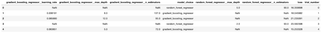
#?我們將首先將每個(gè)試驗(yàn)轉(zhuǎn)換為一個(gè)系列，然后將這些系列堆疊在一起作為一個(gè)數(shù)據(jù)框架。
trials_df?=?pd.DataFrame([pd.Series(t["misc"]["vals"]).apply(unpack)?for?t?in?trials])
#?然后，我們將添加其他相關(guān)的信息到正確的行，并執(zhí)行一些方便的映射
trials_df["loss"]?=?[t["result"]["loss"]?for?t?in?trials]
trials_df["trial_number"]?=?trials_df.index
trials_df[MODEL_CHOICE]?=?trials_df[MODEL_CHOICE].apply(
????lambda?x:?RANDOM_FOREST_REGRESSOR?if?x?==?0?else?GRADIENT_BOOSTING_REGRESSOR

我們?cè)倏匆幌逻@種新格式的前五個(gè)試驗(yàn)：

這比我們之前的字典列表更易于管理。

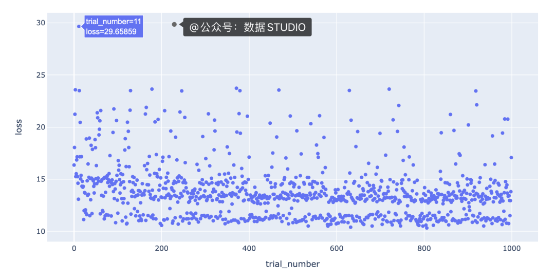
使用 Plotly Express 繪制試驗(yàn)數(shù)量與損失

可視化試驗(yàn)迭代的一種有用方法是繪制試驗(yàn)次數(shù)與損失的關(guān)系圖，以查看超參數(shù)優(yōu)化是否如我們預(yù)期的那樣隨時(shí)間收斂。使用 Plotly 的高級(jí)Express^[3]界面使這變得容易；我們只需在我們的數(shù)據(jù)幀上調(diào)用scatter方法并指出我們想要使用哪些列作為 x 和 y 值：

#?px是“express”的別名，它是按照導(dǎo)入“express”的約定通過運(yùn)行
#?“from plotly import express as px”創(chuàng)建的。
fig?=?px.scatter(trials_df,?x="trial_number",?y="loss")

該圖的一個(gè)有趣特征是，底行具有“損失”值在 10 到 12 之間的點(diǎn)與其余點(diǎn)之間存在明顯的分隔。我們需要更多信息來了解導(dǎo)致這種分離的原因。一種假設(shè)是分離是由不同的模型類型引起的；例如，底行的點(diǎn)可能都是梯度提升回歸模型，其余的點(diǎn)可能都是隨機(jī)森林回歸模型。

我們對(duì)每種模型類型的點(diǎn)進(jìn)行不同的著色，以查看是否是這種情況，方法是color在方法調(diào)用中添加一個(gè)參數(shù)，scatter如下所示：

fig?=?px.scatter(trials_df,?
?????????????????x="trial_number",?
?????????????????y="loss",
?????????????????color=MODEL_CHOICE)

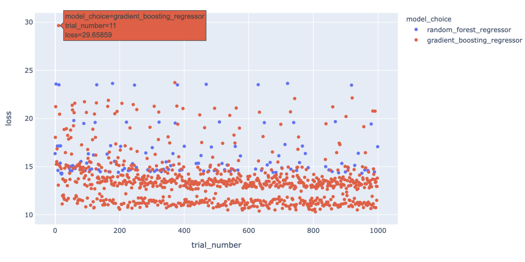
有趣的是，我們看到模型類型并不能完全解釋底行點(diǎn)與其余點(diǎn)之間的差距，因?yàn)樘荻忍嵘貧w模型也出現(xiàn)在其余點(diǎn)中。

我們可以通過創(chuàng)建交互式可視化來為可視化中的信息添加更多深度，這樣當(dāng)我們將鼠標(biāo)懸停在每個(gè)點(diǎn)上時(shí)，我們可以看到導(dǎo)致該點(diǎn)丟失的一組超參數(shù)。起初，看起來我們應(yīng)該能夠通過簡(jiǎn)單地為hover_datascatter 方法的參數(shù)包含一個(gè)值來實(shí)現(xiàn)這一點(diǎn)。但是，由于我們只想為每個(gè)點(diǎn)包含與每種模型類型相關(guān)的超參數(shù)，因此我們需要在update_trace調(diào)用 scatter 之后調(diào)用該方法以添加懸停數(shù)據(jù)，因?yàn)檫@允許我們過濾為每個(gè)點(diǎn)顯示哪些超參數(shù)觀點(diǎn)。看起來是這樣的

我們可以通過這些額外的細(xì)節(jié)來說明什么？將鼠標(biāo)懸停在與底行中最佳模型相對(duì)應(yīng)的點(diǎn)上，可以發(fā)現(xiàn)max_depth每個(gè)點(diǎn)的參數(shù)設(shè)置為3。

此外，將鼠標(biāo)懸停在該行之外的點(diǎn)上會(huì)顯示參數(shù)max_depth設(shè)置為3以外的值，例如2、4或5。這表明在我們的數(shù)據(jù)集中，參數(shù)max_depth可能有一些特殊之處。例如，這可能表明模型性能主要由三個(gè)特征驅(qū)動(dòng)。我們將希望進(jìn)一步研究為什么max_depth=3對(duì)我們的數(shù)據(jù)集如此有效，并且我們可能希望為我們構(gòu)建和部署的最終模型將max_depth設(shè)置為3。

在特征之間創(chuàng)建等高線圖

另一個(gè)可以提高我們對(duì)超參數(shù)設(shè)置直覺的可視化是根據(jù)超參數(shù)的“損失”值的等高線圖。等高線圖特別強(qiáng)大，因?yàn)樗鼈兘沂玖瞬煌瑓?shù)設(shè)置之間的交互如何影響損失。通常，我們希望為每對(duì)超參數(shù)生成一個(gè)單獨(dú)的等高線圖。在這種情況下，為了簡(jiǎn)單起見，我們max_depth將超參數(shù)的值固定為 3，并繪制該數(shù)據(jù)切片的learning_ratevs.n_estimatorsloss 等值線。我們可以通過運(yùn)行以下命令使用 Plotly 創(chuàng)建這個(gè)等高線圖：

#?plotly?express不支持輪廓圖，
#?所以我們將使用'graph_objects'來代替。
#?`go.Contour`自動(dòng)為我們的損失插入“z”值。
fig?=?go.Figure(
????data=go.Contour(
????????z=trials_df.loc[max_depth_filter,?"loss"],
????????x=trials_df.loc[max_depth_filter,?"gradient_boosting_regressor__learning_rate"],
????????y=trials_df.loc[max_depth_filter,?"gradient_boosting_regressor__n_estimators"],
????????contours=dict(
????????????showlabels=True,??#?顯示輪廓上的標(biāo)簽
????????????labelfont=dict(size=12,?color="white",),??
????????????#?標(biāo)簽字體屬性
????????),
????????colorbar=dict(title="loss",?titleside="right",),
????????hovertemplate="loss:?%{z}
learning_rate:?%{x}
n_estimators:?%{y}",
????)
)

fig.update_layout(
????xaxis_title="learning_rate",
????yaxis_title="n_estimators",
????title={
????????"text":?"learning_rate?vs.?n_estimators?|?max_depth?==?3",
????????"xanchor":?"center",
????????"yanchor":?"top",
????????"x":?0.5,
????},
)

該圖的一個(gè)要點(diǎn)是，我們可能希望嘗試增加最大值n_estimators超參數(shù)，因?yàn)閾p失最低的區(qū)域出現(xiàn)在該圖的頂部。

寫在最后

在這篇文章中，我們介紹了如何將試驗(yàn)對(duì)象中包含的數(shù)據(jù)轉(zhuǎn)換為 Pandas 數(shù)據(jù)框，以便我們可以輕松分析超參數(shù)設(shè)置的歷史。一旦我們?cè)跀?shù)據(jù)框中獲得了數(shù)據(jù)，我們就可以輕松地創(chuàng)建可視化，讓我們更好地了解為什么一組特定的超參數(shù)設(shè)置是最好的。特別是，我們已經(jīng)證明，通過使用 Plotly 創(chuàng)建簡(jiǎn)單的交互式可視化來增加可視化的深度，可以揭示一些非常適合我們的問題的超參數(shù)設(shè)置的有趣趨勢(shì)。此外，我們已經(jīng)展示了等高線圖對(duì)于指示我們可能想要對(duì)超參數(shù)搜索空間進(jìn)行的調(diào)整很有用。


長(zhǎng)按或掃描下方二維碼，后臺(tái)回復(fù)：加群，即可申請(qǐng)入群。一定要備注：來源+研究方向+學(xué)校/公司，否則不拉入群中，見諒！
（長(zhǎng)按三秒，進(jìn)入后臺(tái)）

推薦閱讀
微軟拆分VS Code Python擴(kuò)展，再推3款獨(dú)立擴(kuò)展！
30 個(gè)Python代碼實(shí)現(xiàn)的常用功能，精心整理版
最該收藏的8款可視化工具，人人都有選擇！
60 個(gè)神級(jí) VS Code 插件！

使用 Hyperopt 和 Plotly 可視化超參數(shù)優(yōu)化