
yyds!用機器學(xué)習(xí)預(yù)測 bilibili 股價走勢


numpy、pandas、matplotlib、scipy等Python數(shù)據(jù)科學(xué)工具包。#關(guān)注公眾號:寬客邦,回復(fù)“源碼”獲取下載本文完整源碼
import numpy as np
import pandas as pd
from math import sqrt
import matplotlib.pyplot as plt
from scipy.stats import norm
from pandas_datareader import data
pd.to_datetime將數(shù)據(jù)集時間轉(zhuǎn)化為時間序列,便于股票的分析。BILI = data.DataReader('BILI', 'yahoo',start='29/3/2018',)
BILI.index=pd.to_datetime(BILI.index)
head()方法看一下數(shù)據(jù)集的結(jié)構(gòu),數(shù)據(jù)集包含了股票的開盤價、收盤價、每日最低價與最高價、交易量等信息。掃描本文最下方二維碼獲取全部完整源碼和Jupyter Notebook 文件打包下載。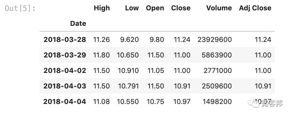
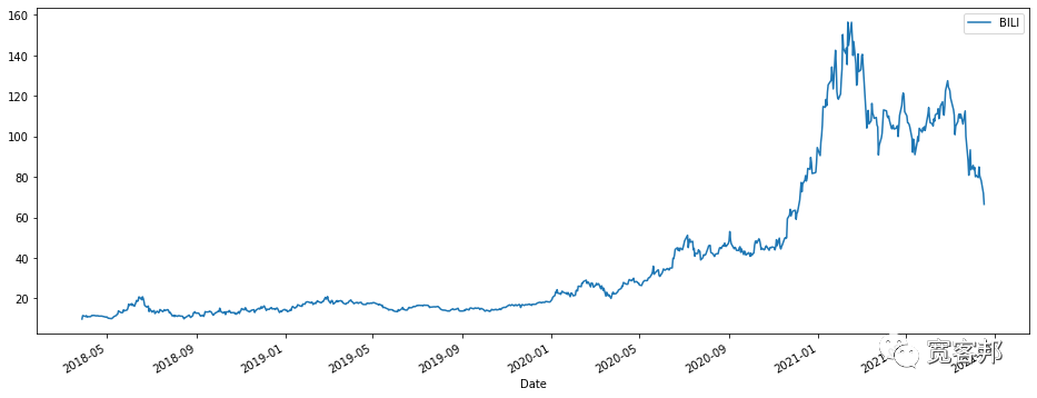
plt.legend用于設(shè)置圖像的圖例,loc是圖例位置,upper right代表圖例在右上角。從圖中可以看出嗶哩嗶哩股票在2020年12月到2021年2月之間有一個快速的增長,隨后股價有所回落。plt.figure(figsize=(16,6))
BILI['Open'].plot()
plt.legend(['BILI'],loc='upper right')
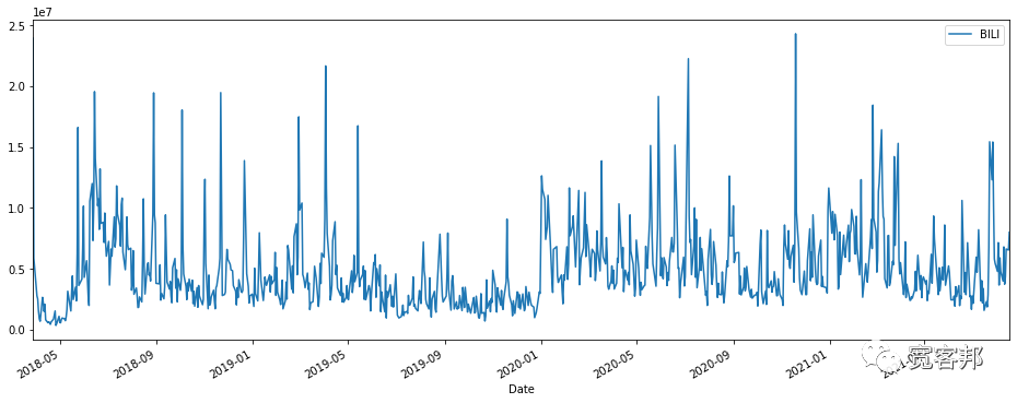
plt.figure(figsize=(16,6))
BILI['Volume'].plot()
plt.legend(['BILI'],loc='upper right')
plt.xlim(BILI.index[0],BILI.index[-1])
BILI['Total Traded']=BILI['Open']*BILI['Volume']

plt.figure(figsize=(16,6))
BILI['Total Traded'].plot()

plt.legend(['BILI'],loc='upper right')
plt.xlim(BILI.index[0],BILI.index[-1])
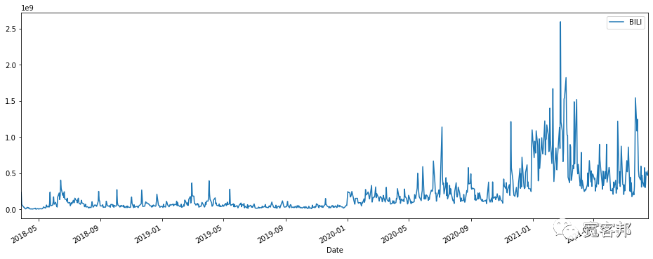
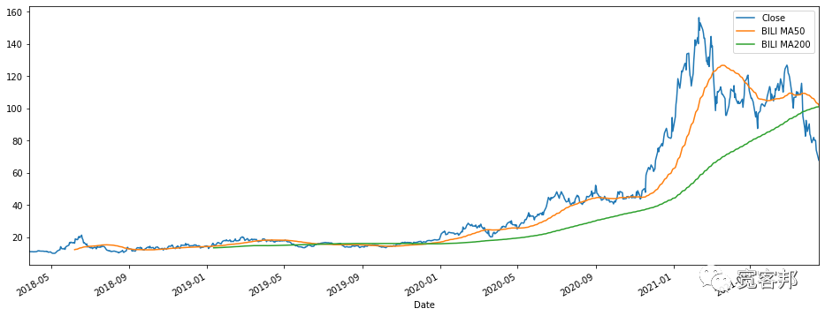
argmax()獲取最大交易總額的日期。BILI['Total Traded'].argmax()Timestamp('2021-02-25 00:00:00')BILI這支股票的收盤價及其移動平均線,我們可以用DataFrame的rolling()函數(shù)得到移動平均值。BILI['Close'].plot(figsize=(16,6),xlim=(BILI.index[0],BILI.index[-1]))
BILI['Close'].rolling(50).mean().plot(label='BILI MA50')
BILI['Close'].rolling(200).mean().plot(label='BILI MA200')
plt.legend()
ffn.to_returns函數(shù)計算;第三種是利用pandas自帶的函數(shù)pct_change(1)進行計算。掃描本文最下方二維碼獲取全部完整源碼和Jupyter Notebook 文件打包下載。#關(guān)注公眾號:寬客邦,回復(fù)“源碼”獲取完整源碼,直接使用計算公式計算
BILI['Return']=(BILI['Close']-BILI['Close'].shift(1))/BILI['Close'].shift(1)
BILI=BILI.dropna()
#導(dǎo)入專用于金融領(lǐng)域的第三方庫ffn.to_returns函數(shù)計算
import ffn
BILI['Return']=ffn.to_returns(BILI['Close'])
#利用pandas自帶的函數(shù)pct_change(1)進行計算
BILI['Return']=BILI['Close'].pct_change()
BILI=BILI.dropna()
#關(guān)注公眾號:寬客邦,回復(fù)“源碼”獲取下載本文完整源碼
plt.hist(BILI['Return'],bins=50)

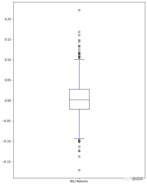
box_df = pd.concat([BILI['Return']],axis=1)
box_df.columns = ['BILI Returns']
box_df.plot(kind='box',figsize=(8,11),colormap='jet')
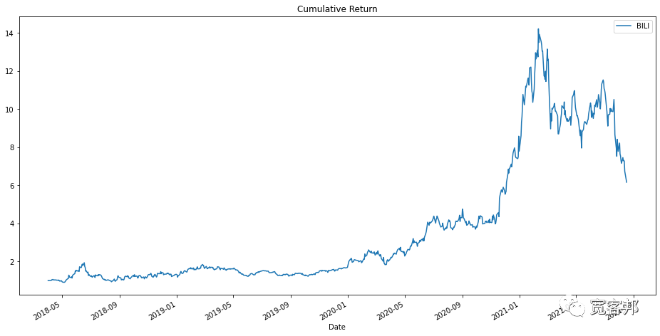
BILI['Cumulative Return']=(1+BILI['Return']).cumprod()

BILI['Cumulative Return'].plot(label='BILI',figsize=(16,8),title='Cumulative Return')
plt.legend()
#關(guān)注公眾號:寬客邦,回復(fù)“源碼”獲取完整源碼,計算復(fù)合年均增長率
days = (BILI.index[-1] - BILI.index[0]).days
cagr = ((((BILI['Adj Close'][-1]) / BILI['Adj Close'][1])) ** (365.0/days)) - 1
print ('CAGR =',str(round(cagr)*100)+"%")
mu = cagr

#計算收益的年度波動率
BILI['Returns'] = BILI['Adj Close'].pct_change()
vol = BILI['Returns']*sqrt(252)
print ("Annual Volatility =",str(round(vol,4)*100)+"%")
CAGR = 71.72%Annual Volatility = 65.14%
S = BILI['Adj Close'][-1] #起始股票價格(即最后一天的實際股票價格)
T = 252 #交易天數(shù)
mu = 0.7172 #復(fù)合年均增長率
vol = 0.6514 #年度波動率
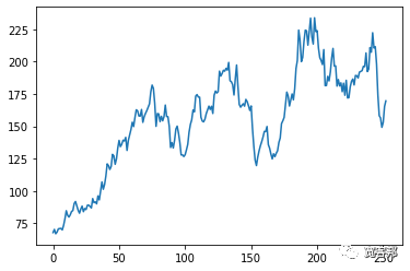
#關(guān)注公眾號:寬客邦,回復(fù)“源碼”獲取完整源碼,使用隨機正態(tài)分布創(chuàng)建每日收益列表
daily_returns=np.random.normal((mu/T),vol/math.sqrt(T))+1
#關(guān)注公眾號:寬客邦,回復(fù)“源碼”獲取下載本文完整源碼
price_list = [S]
for x in daily_returns:
price_list.append(price_list[-1]*x)
#生成價格序列的折線圖
plt.plot(price_list)
plt.show()
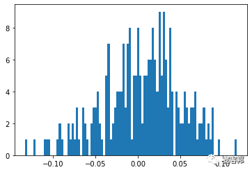
plt.hist(daily_returns-1, 100)
plt.show()
import numpy as np
import math
import matplotlib.pyplot as plt
from scipy.stats import norm
#關(guān)注公眾號:寬客邦,回復(fù)“源碼”獲取下載本文完整源碼
S = BILI['Adj Close'][-1] #起始股票價格(即最后一天的實際股票價格)
T = 252 #交易天數(shù)
mu = 0.7172 #復(fù)合年均增長率
vol = 0.6514 #年度波動率
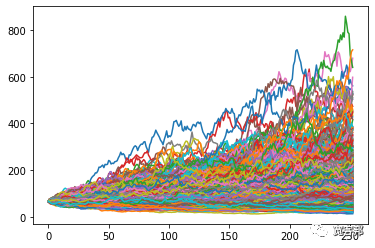
#選擇要模擬的運行次數(shù) - 我選擇1000
for i in range(1000):
#使用隨機正態(tài)分布創(chuàng)建每日收益列表
daily_returns=np.random.normal(mu/T,vol/math.sqrt(T))+1
#設(shè)置起始價格并創(chuàng)建由上述隨機每日收益生成的價格列表
price_list = [S]
for x in daily_returns:
price_list.append(price_list[-1]*x)
#繪制來自每個單獨運行的數(shù)據(jù),我們將在最后繪制
plt.plot(price_list)
#顯示上面創(chuàng)建的多個價格系列的圖
plt.show()
import numpy as np
import math
import matplotlib.pyplot as plt
from scipy.stats import norm
#關(guān)注公眾號:寬客邦,回復(fù)“源碼”獲取下載本文完整源碼
result = []
#定義變量
S = BILI['Adj Close'][-1] #起始股票價格(即最后一天的實際股票價格)
T = 252 #交易天數(shù)
mu = 0.7172 #復(fù)合年均增長率
vol = 0.6514 #年度波動率
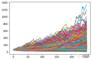
#選擇要模擬的運行次數(shù) - 選擇10000
for i in range(10000):
#使用隨機正態(tài)分布創(chuàng)建每日收益列表
daily_returns=np.random.normal(mu/T,vol/math.sqrt(T))+1
#設(shè)置起始價格并創(chuàng)建由上述隨機每日收益生成的價格列表
price_list = [S]
for x in daily_returns:
price_list.append(price_list[-1]*x)
#繪制來自每個單獨運行的數(shù)據(jù),我們將在最后繪制
plt.plot(price_list)
#將每次模擬運行的結(jié)束值附加到我們在開始時創(chuàng)建的空列表中
result.append(price_list[-1])
#顯示上面創(chuàng)建的多個價格系列的圖
plt.show()
plt.hist(result,bins=50)
plt.show()
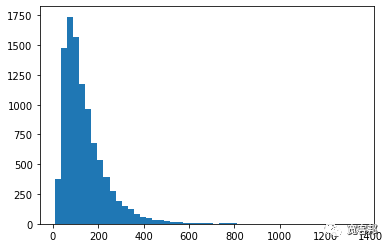
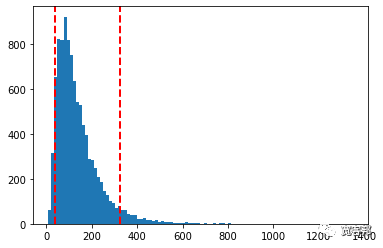
numpy mean函數(shù)計算平均值的分布,以獲得我們的“預(yù)期值”。print(round(np.mean(result)))
139.18print("5% quantile =",np.percentile(result,5))
print("95% quantile =",np.percentile(result,95))
5% quantile = 38.33550814175252
95% quantile = 326.44060907630484
plt.hist(result,bins=100)
plt.axvline(np.percentile(result,5), color='r', linestyle='dashed')
plt.axvline(np.percentile(result,95), color='r', linestyle='dashed')
plt.show()
↓↓長按掃碼獲取完整源碼↓↓
評論
圖片
表情