
使用直方圖處理進(jìn)行顏色校正
點(diǎn)擊上方“小白學(xué)視覺”,選擇加"星標(biāo)"或“置頂”
重磅干貨,第一時間送達(dá)

在這篇文章中,我們將探討如何使用直方圖處理技術(shù)來校正圖像中的顏色。
像往常一樣,我們導(dǎo)入庫,如numpy和matplotlib。此外,我們還從skimage 和scipy.stats庫中導(dǎo)入特定函數(shù)。
import numpy as npimport matplotlib.pyplot as pltfrom skimage.io import imread, imshowfrom skimage import img_as_ubytefrom skimage.color import rgb2grayfrom skimage.exposure import histogram, cumulative_distributionfrom scipy.stats import cauchy, logistic
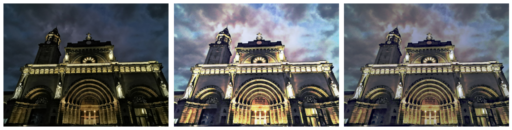
讓我們使用馬尼拉內(nèi)穆羅斯馬尼拉大教堂的夜間圖像。
cathedral = imread('cathedral.jpg')plt.imshow(cathedral)plt.title('Manila Cathedral')
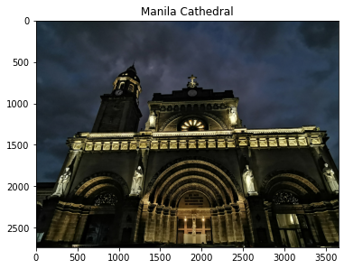
首先,讓我們將圖像轉(zhuǎn)換為灰度。
fig, ax = plt.subplots(1,2, figsize=(15,5))cathedral_gray = rgb2gray(cathedral)ax[0].imshow(cathedral_gray, cmap='gray')ax[0].set_title('Grayscale Image')ax1 = ax[1]ax2 = ax1.twinx()freq_h, bins_h = histogram(cathedral_gray)freq_c, bins_c = cumulative_distribution(cathedral_gray)ax1.step(bins_h, freq_h*1.0/freq_h.sum(), c='b', label='PDF')ax2.step(bins_c, freq_c, c='r', label='CDF')ax1.set_ylabel('PDF', color='b')ax2.set_ylabel('CDF', color='r')ax[1].set_xlabel('Intensity value')ax[1].set_title('Histogram of Pixel Intensity');
由于圖像是在夜間拍攝的,因此圖像的特征比較模糊,這也在像素強(qiáng)度值的直方圖上觀察到,其中 PDF 在較低的光譜上偏斜。
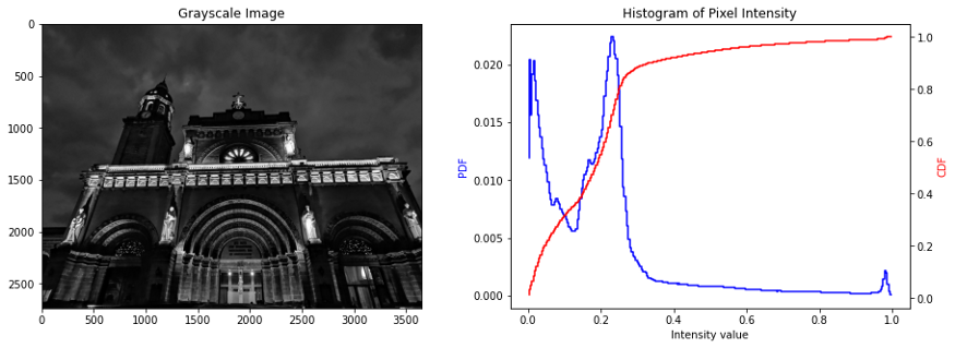
由于圖像的強(qiáng)度值是傾斜的,因此可以應(yīng)用直方圖處理來重新分布圖像的強(qiáng)度值。直方圖處理的目的是將圖像的實(shí)際 CDF 拉伸到新的目標(biāo) CDF 中。通過這樣做,傾斜到較低光譜的強(qiáng)度值將轉(zhuǎn)換為較高的強(qiáng)度值,從而使圖像變亮。
讓我們嘗試在灰度圖像上實(shí)現(xiàn)這一點(diǎn),我們假設(shè) PDF 是均勻分布,CDF 是線性分布。
image_intensity = img_as_ubyte(cathedral_gray)freq, bins = cumulative_distribution(image_intensity)target_bins = np.arange(255)target_freq = np.linspace(0, 1, len(target_bins))new_vals = np.interp(freq, target_freq, target_bins)fig, ax = plt.subplots(1,2, figsize=(15,5))ax[0].step(bins, freq, c='b', label='Actual CDF')ax[0].plot(target_bins, target_freq, c='r', label='Target CDF')ax[0].legend()ax[0].set_title('Grayscale: Actual vs. ''Target Cumulative Distribution')ax[1].imshow(new_vals[image_intensity].astype(np.uint8),cmap='gray')ax[1].set_title('Corrected?Image?in?Grayscale');
通過將實(shí)際 CDF 轉(zhuǎn)換為目標(biāo) CDF,我們可以在保持圖像關(guān)鍵特征的同時使圖像變亮。請注意,這與僅應(yīng)用亮度過濾器完全不同,因?yàn)榱炼冗^濾器只是將圖像中所有像素的強(qiáng)度值增加相等的量。在直方圖處理中,像素強(qiáng)度值可以根據(jù)目標(biāo) CDF 增加或減少。
現(xiàn)在,讓我們嘗試在彩色圖像中實(shí)現(xiàn)直方圖處理。這些過程可以從灰度圖像中復(fù)制——然而,不同之處在于我們需要對圖像的每個通道應(yīng)用直方圖處理。為了簡化實(shí)現(xiàn),我們創(chuàng)建一個函數(shù)來對圖像執(zhí)行此過程。
def show_linear_cdf(image, channel, name, ax):image_intensity = img_as_ubyte(image[:,:,channel])freq, bins = cumulative_distribution(image_intensity)target_bins = np.arange(255)target_freq = np.linspace(0, 1, len(target_bins))ax.step(bins, freq, c='b', label='Actual CDF')ax.plot(target_bins, target_freq, c='r', label='Target CDF')ax.legend()ax.set_title('{} Channel: Actual vs. ''Target Cumulative Distribution'.format(name))def linear_distribution(image, channel):image_intensity = img_as_ubyte(image[:,:,channel])freq, bins = cumulative_distribution(image_intensity)target_bins = np.arange(255)target_freq = np.linspace(0, 1, len(target_bins))new_vals = np.interp(freq, target_freq, target_bins)return new_vals[image_intensity].astype(np.uint8)
現(xiàn)在,我們將這些函數(shù)應(yīng)用于原始圖像的每個通道。
fig, ax = plt.subplots(3,2, figsize=(12,14))red_channel = linear_distribution(cathedral, 0)green_channel = linear_distribution(cathedral, 1)blue_channel = linear_distribution(cathedral, 2)show_linear_cdf(cathedral, 0, ‘Red’, ax[0,0])ax[0,1].imshow(red_channel, cmap=’Reds’)ax[0,1].set_title(‘Corrected Image in Red Channel’)show_linear_cdf(cathedral, 1, ‘Green’, ax[1,0])ax[1,1].imshow(green_channel, cmap=’Greens’)ax[1,1].set_title(‘Corrected Image in Green Channel’)show_linear_cdf(cathedral, 2, ‘Blue’, ax[2,0])ax[2,1].imshow(blue_channel, cmap=’Blues’)ax[2,1].set_title(‘Corrected Image in Blue Channel’)
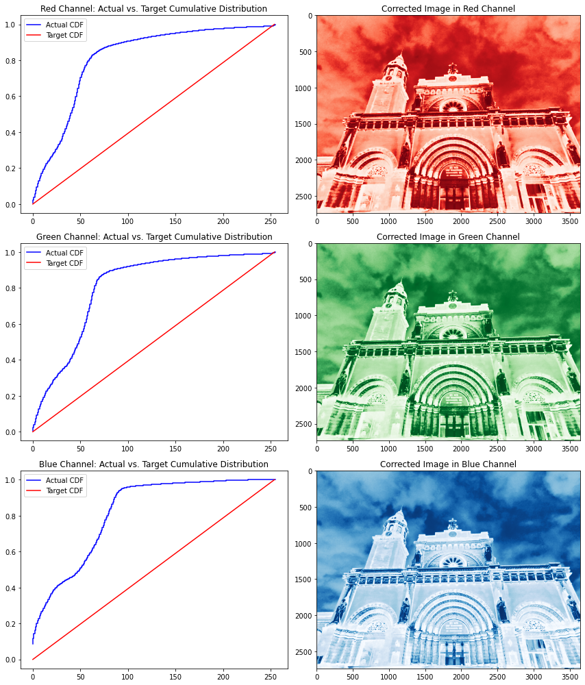
請注意,所有通道幾乎都具有相同的 CDF,這顯示了圖像中顏色的良好分布——只是顏色集中在較低的強(qiáng)度值光譜上。就像我們在灰度圖像中所做的一樣,我們還將每個通道的實(shí)際 CDF 轉(zhuǎn)換為目標(biāo) CDF。
校正每個通道的直方圖后,我們需要使用 numpy stack函數(shù)將這些通道堆疊在一起。請注意,RGB 通道在堆疊時需要按順序排列。
fig, ax = plt.subplots(1,2, figsize=(15,5))ax[0].imshow(cathedral);ax[0].set_title('Original Image')ax[1].imshow(np.dstack([red_channel, green_channel, blue_channel]));ax[1].set_title('Transformed Image');
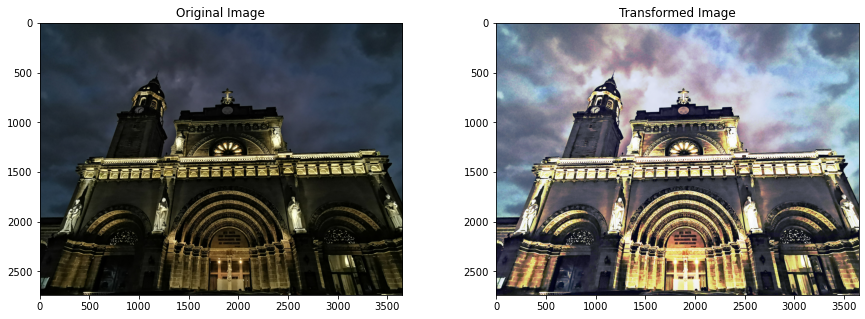
堆疊所有通道后,我們可以看到轉(zhuǎn)換后的圖像顏色與原始圖像的顯著差異。直方圖處理最有趣的地方在于,圖像的不同部分會有不同程度的像素強(qiáng)度轉(zhuǎn)換。請注意,馬尼拉大教堂墻壁的像素強(qiáng)度發(fā)生了巨大變化,而馬尼拉大教堂鐘樓的像素強(qiáng)度卻保持相對不變。
現(xiàn)在,讓我們嘗試使用其他函數(shù)作為目標(biāo) CDF 來改進(jìn)這一點(diǎn)。為此,我們將使用該scipy.stats庫導(dǎo)入各種分布,還創(chuàng)建了一個函數(shù)來簡化我們的分析。
def individual_channel(image, dist, channel):im_channel = img_as_ubyte(image[:,:,channel])freq, bins = cumulative_distribution(im_channel)new_vals = np.interp(freq, dist.cdf(np.arange(0,256)),np.arange(0,256))return new_vals[im_channel].astype(np.uint8)def distribution(image, function, mean, std):dist = function(mean, std)fig, ax = plt.subplots(1,2, figsize=(15,5))image_intensity = img_as_ubyte(rgb2gray(image))freq, bins = cumulative_distribution(image_intensity)ax[0].step(bins, freq, c='b', label='Actual CDF')ax[0].plot(dist.cdf(np.arange(0,256)),c='r', label='Target CDF')ax[0].legend()ax[0].set_title('Actual vs. Target Cumulative Distribution')red = individual_channel(image, dist, 0)green = individual_channel(image, dist, 1)blue = individual_channel(image, dist, 2)ax[1].imshow(np.dstack((red, green, blue)))ax[1].set_title('Transformed Image')return ax
讓我們使用 Cauchy 函數(shù)來試試這個。
distribution(cathedral, cauchy, 90, 30);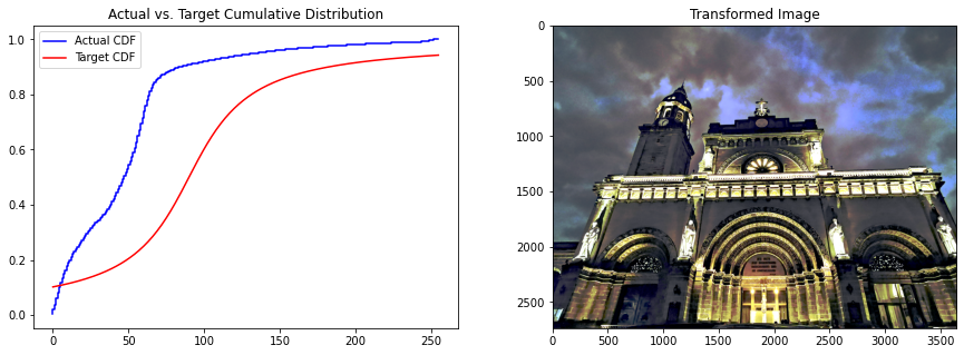
使用不同的分布似乎會產(chǎn)生更令人愉悅的配色方案。事實(shí)上,大教堂正門的弧線在邏輯分布中比線性分布更好,這是因?yàn)樵谶壿嫹植贾邢袼刂祻?qiáng)度的平移比線性分布要小,這可以從實(shí)際 CDF 線到目標(biāo) CDF 線的距離看出。
讓我們看看我們是否可以使用邏輯分布進(jìn)一步改進(jìn)這一點(diǎn)。
distribution(cathedral, logistic, 90, 30);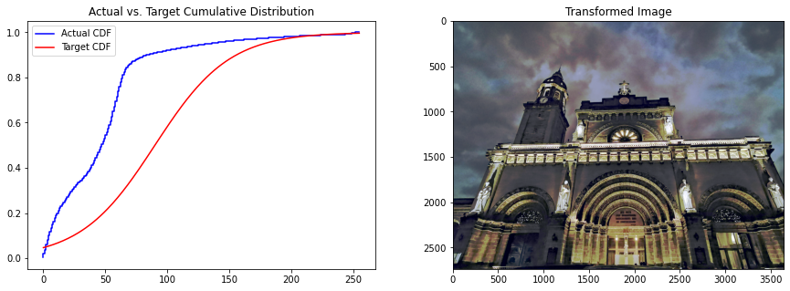
請注意,門中的燈光如何從線性和Cauchy分布改進(jìn)為邏輯分布的。這是因?yàn)檫壿嫼瘮?shù)的上譜幾乎與原始 CDF 一致。因此,圖像中的所有暗物體(低像素強(qiáng)度值)都被平移,而燈光(高像素強(qiáng)度值)幾乎保持不變。
我們已經(jīng)探索了如何使用直方圖處理來校正圖像中的顏色,實(shí)現(xiàn)了各種分布函數(shù),以了解它如何影響結(jié)果圖像中的顏色分布。
同樣,我們可以得出結(jié)論,在固定圖像的顏色強(qiáng)度方面沒有“一體適用”的解決方案,數(shù)據(jù)科學(xué)家的主觀決定是確定哪個是最適合他們的圖像處理需求的解決方案。
Github代碼連接:
https://github.com/jephraim-manansala/histogram-manipulation
交流群
歡迎加入公眾號讀者群一起和同行交流,目前有SLAM、三維視覺、傳感器、自動駕駛、計算攝影、檢測、分割、識別、醫(yī)學(xué)影像、GAN、算法競賽等微信群(以后會逐漸細(xì)分),請掃描下面微信號加群,備注:”昵稱+學(xué)校/公司+研究方向“,例如:”張三?+?上海交大?+?視覺SLAM“。請按照格式備注,否則不予通過。添加成功后會根據(jù)研究方向邀請進(jìn)入相關(guān)微信群。請勿在群內(nèi)發(fā)送廣告,否則會請出群,謝謝理解~