
(附代碼)實戰(zhàn) | 基于深度學(xué)習(xí)的道路損壞檢測
點擊左上方藍字關(guān)注我們

道路基礎(chǔ)設(shè)施是一項重要的公共資產(chǎn),因為它有助于經(jīng)濟發(fā)展和增長,同時帶來重要的社會效益。路面檢查主要基于人類的視覺觀察和使用昂貴機器的定量分析。這些方法的最佳替代方案是智能探測器,它使用記錄的圖像或視頻來檢測損壞情況。除了道路INFR一個結(jié)構(gòu),道路破損檢測器也將在自主駕駛汽車,以檢測他們的方式有些坑洼或其他干擾,盡量避免他們有用。
本項目中使用的數(shù)據(jù)集是從這里收集的。該數(shù)據(jù)集包含不同國家的道路圖像,它們是日本、印度、捷克。對于圖像,標(biāo)簽的注釋是在 xml 文件中,即標(biāo)簽是 PASCAL VOC 格式。由于數(shù)據(jù)集包含來自日本的大部分圖像(在以前的版本中,它僅包含來自日本的圖像),因此根據(jù)數(shù)據(jù)來源,根據(jù)日本道路指南確定了標(biāo)簽。
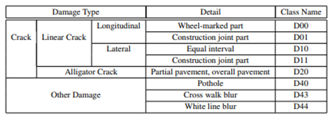
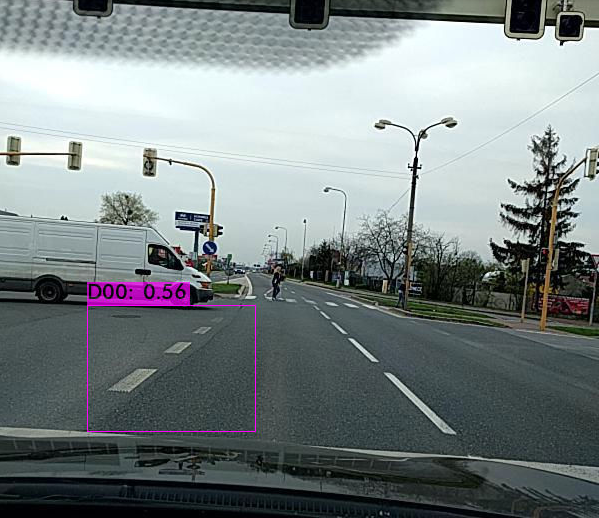
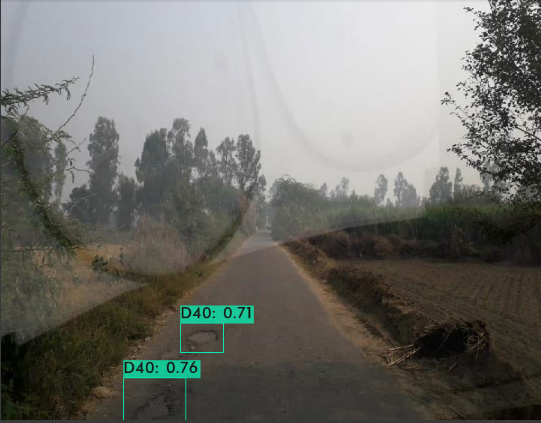
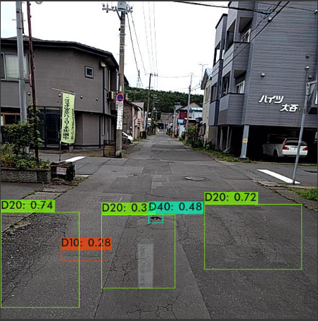
但是最新的數(shù)據(jù)集現(xiàn)在包含其他國家的圖像,因此為了概括我們只考慮以下標(biāo)簽的損害。D00:垂直裂縫,D10:水平裂縫,D20:鱷魚裂縫,D40:坑洼
CNN 或卷積神經(jīng)網(wǎng)絡(luò)是所有計算機視覺任務(wù)的基石。即使在物體檢測的情況下,從圖像中提取物體的模式到特征圖(基本上是一個比圖像尺寸小的矩陣)卷積操作也被使用。現(xiàn)在從過去幾年開始,已經(jīng)對對象檢測任務(wù)進行了大量研究,我們得到了大量最先進的算法或方法,其中一些簡而言之,我們在下面進行了解釋。
數(shù)據(jù)集中的圖像總數(shù):26620
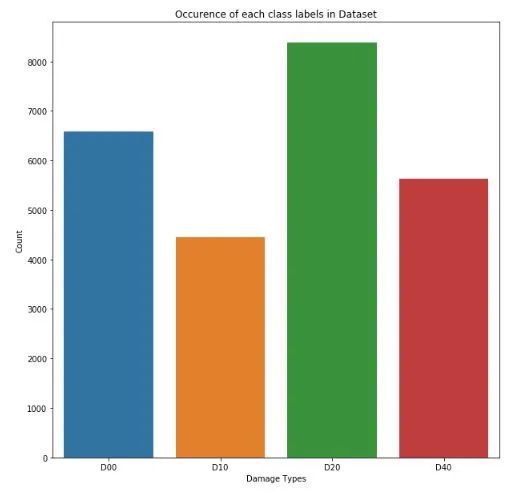
標(biāo)簽分布
每個班級的計數(shù)D00 : 6592D10 : 4446D20 : 8381: 5627
各國標(biāo)簽分布(全數(shù)據(jù)分析)
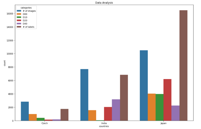
捷克數(shù)據(jù)分析0 圖像數(shù)量 28291 D00 9882 D10 3993 D20 1614 D40 1975 標(biāo)簽數(shù)量 1745************************ **********************************************印度數(shù)據(jù)分析類別計數(shù)6 圖像數(shù)量 77067 D00 15558 D10 689 D20 202110 D40 318711 標(biāo)簽數(shù)量 6831**************************** ******************************************日本數(shù)據(jù)分析12 圖像數(shù)量 1050613 D00 404914 D10 397915 D20 619916 D40 224317 標(biāo)簽數(shù)量 16470************************************ ************************************
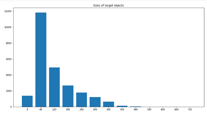
圖像中標(biāo)簽大小的分布
標(biāo)簽最小尺寸:0x1 標(biāo)簽最大尺寸:704x492
對象檢測現(xiàn)在是一個龐大的主題,相當(dāng)于一個學(xué)期的主題。它由許多算法組成。因此,為了使其簡短,目標(biāo)檢測算法被分為各種類別,例如基于區(qū)域的算法(RCNN、Fast-RCNN、Faster-RCNN)、兩級檢測器、一級檢測器,其中基于區(qū)域的算法本身是兩級檢測器的一部分,但我們將在下面簡要地解釋它們,因此我們明確地提到了它們。讓我們從RCNN(基于區(qū)域的卷積神經(jīng)網(wǎng)絡(luò))開始。
目標(biāo)檢測算法的基本架構(gòu)由兩部分組成。該部分由一個 CNN 組成,它將原始圖像信息轉(zhuǎn)換為特征圖,在下一部分中,不同的算法有不同的技術(shù)。因此,在 RCNN 的情況下,它使用選擇性搜索來獲得 ROI(感興趣區(qū)域),即在那個地方有可能有不同的對象。從每個圖像中提取大約 2000 個區(qū)域。它使用這些 ROI 對標(biāo)簽進行分類并使用兩種不同的模型預(yù)測對象位置。因此這些模型被稱為兩級檢測器。
RCNN 有一些限制,為了克服這些限制,他們提出了 Fast RCNN。RCNN 具有很高的計算時間,因為每個區(qū)域都分別傳遞給 CNN,并且它使用三種不同的模型進行預(yù)測。因此,在 Fast RCNN 中,每個圖像只傳遞一次到 CNN 并提取特征圖。在這些地圖上使用選擇性搜索來生成預(yù)測。將 RCNN 中使用的所有三個模型組合在一起。
但是 Fast RCNN 仍然使用緩慢的選擇性搜索,因此計算時間仍然很長。猜猜他們想出了另一個名字有意義的版本,即更快的 RCNN。Faster RCNN 用區(qū)域提議網(wǎng)絡(luò)代替了選擇性搜索方法,使算法更快。現(xiàn)在讓我們轉(zhuǎn)向一些一次性檢測器。YOLO 和 SSD 是非常著名的物體檢測模型,因為它們在速度和準(zhǔn)確性之間提供了非常好的權(quán)衡
YOLO:單個神經(jīng)網(wǎng)絡(luò)在一次評估中直接從完整圖像中預(yù)測邊界框和類別概率。由于整個檢測管道是一個單一的網(wǎng)絡(luò),因此可以直接在檢測性能上進行端到端的優(yōu)化
SSD(Single Shot Detector):SSD 方法將邊界框的輸出空間離散為一組不同縱橫比的默認框。離散化后,該方法按特征圖位置進行縮放。Single Shot Detector 網(wǎng)絡(luò)結(jié)合了來自具有不同分辨率的多個特征圖的預(yù)測,以自然地處理各種大小的對象。
作為深度學(xué)習(xí)的新手,或者準(zhǔn)確地說是計算機視覺,為了學(xué)習(xí)基礎(chǔ)知識,我們嘗試了一些基本且快速的算法來實現(xiàn)如下數(shù)據(jù)集:
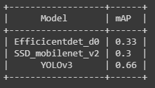
Efficientdet_d0SSD_mobilenet_v2YOLOv3
對于第一個和第二個模型,我們使用了tensorflow 模型 zoo并且為了訓(xùn)練 yolov3 引用了this。用于評估 mAP(平均平均精度),使用 Effectivedet_d0 和 ssd_mobilenet_v2 得到的 mAP 非常低,可能是因為沒有更改學(xué)習(xí)率、優(yōu)化器和數(shù)據(jù)增強的一些默認配置。
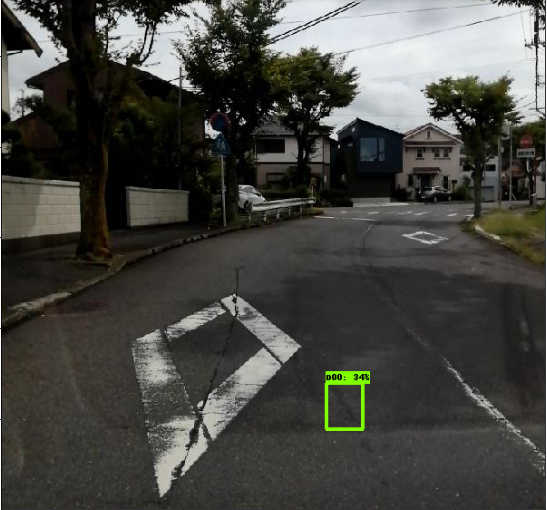
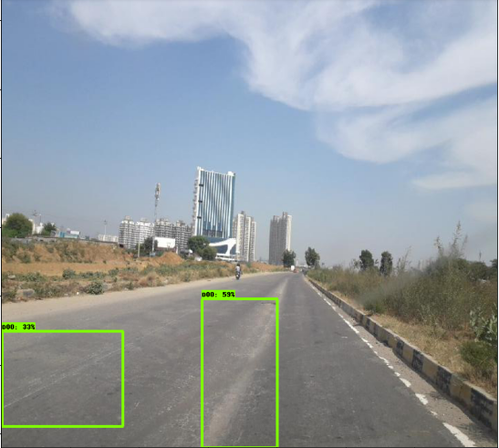
使用 efficicentdet_d0 進行推導(dǎo)
import tensorflow as tffrom object_detection.utils import label_map_utilfrom object_detection.utils import config_utilfrom object_detection.utils import visualization_utils as viz_utilsfrom object_detection.builders import model_builder# Load pipeline config and build a detection modelconfigs = config_util.get_configs_from_pipeline_file('/content/efficientdet_d0_coco17_tpu-32/pipeline.config')model_config = configs['model']detection_model = model_builder.build(model_config=model_config, is_training=False)# Restore checkpointckpt = tf.compat.v2.train.Checkpoint(model=detection_model)ckpt.restore('/content/drive/MyDrive/efficientdet/checkpoints/ckpt-104').expect_partial()def detect_fn(image):"""Detect objects in image."""image, shapes = detection_model.preprocess(image)prediction_dict = detection_model.predict(image, shapes)detections = detection_model.postprocess(prediction_dict, shapes)return detectionscategory_index = label_map_util.create_category_index_from_labelmap('/content/data/label_map.pbtxt',use_display_name=True)for image_path in IMAGE_PATHS:print('Running inference for {}... '.format(image_path), end='')image_np = load_image_into_numpy_array(image_path)input_tensor = tf.convert_to_tensor(np.expand_dims(image_np, 0), dtype=tf.float32)detections = detect_fn(input_tensor)num_detections = int(detections.pop('num_detections'))detections = {key: value[0, :num_detections].numpy()for key, value in detections.items()}detections['num_detections'] = num_detections# detection_classes should be ints.detections['detection_classes'] = detections['detection_classes'].astype(np.int64)label_id_offset = 1image_np_with_detections = image_np.copy()viz_utils.visualize_boxes_and_labels_on_image_array(image_np_with_detections,detections['detection_boxes'],detections['detection_classes']+label_id_offset,detections['detection_scores'],category_index,use_normalized_coordinates=True,max_boxes_to_draw=200,min_score_thresh=.30,agnostic_mode=False)%matplotlib inlinefig = plt.figure(figsize = (10,10))plt.imshow(image_np_with_detections)print('Done')plt.show()
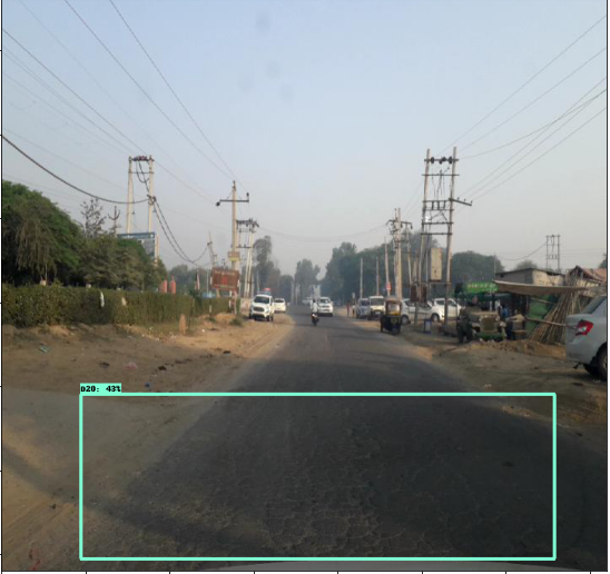
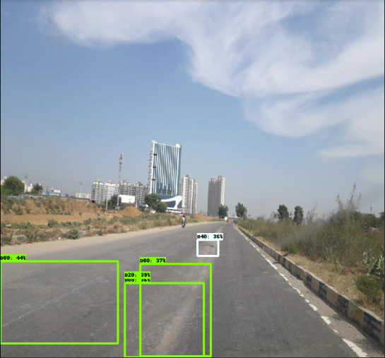
使用 SSD_mobilenet_v2 進行推導(dǎo)
(與efficientdet 相同的代碼)
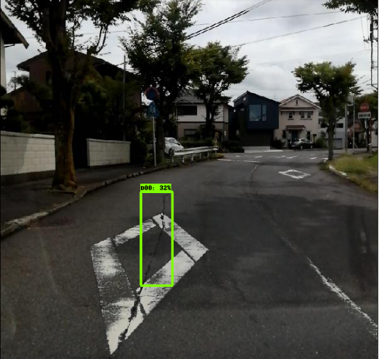
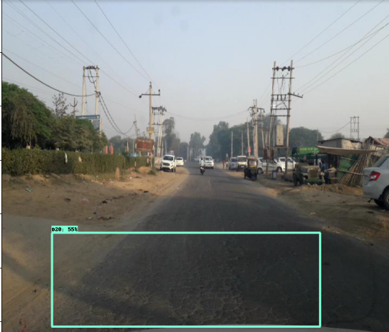
YOLOv3 的推導(dǎo)
def func(input_file):classes = ['D00', 'D10', 'D20', 'D40']alt_names = {'D00': 'lateral_crack', 'D10': 'linear_cracks', 'D20': 'aligator_crakcs', 'D40': 'potholes'}# initialize a list of colors to represent each possible class labelnp.random.seed(42)COLORS = np.random.randint(0, 255, size=(len(classes), 3),dtype="uint8")# derive the paths to the YOLO weights and model configurationweightsPath = "/content/drive/MyDrive/yolo/yolo-obj_final.weights"configPath = "/content/yolov3.cfg"# load our YOLO object detector trained on COCO dataset (80 classes)# and determine only the *output* layer names that we need from YOLO#print("[INFO] loading YOLO from disk...")net = cv2.dnn.readNetFromDarknet(configPath, weightsPath)ln = net.getLayerNames()ln = [ln[i[0] - 1] for i in net.getUnconnectedOutLayers()]# read the next frame from the fileframe = cv2.imread(input_file)W) = frame.shape[:2]# construct a blob from the input frame and then perform a forward# pass of the YOLO object detector, giving us our bounding boxes# and associated probabilitiesblob = cv2.dnn.blobFromImage(frame, 1 / 255.0, (416, 416),swapRB=True, crop=False)net.setInput(blob)start = time.time()layerOutputs = net.forward(ln)end = time.time()# initialize our lists of detected bounding boxes, confidences,# and class IDs, respectivelyboxes = []confidences = []classIDs = []# loop over each of the layer outputsfor output in layerOutputs:# loop over each of the detectionsfor detection in output:# extract the class ID and confidence (i.e., probability)# of the current object detectionscores = detection[5:]classID = np.argmax(scores)confidence = scores[classID]# filter out weak predictions by ensuring the detected# probability is greater than the minimum probabilityif confidence > 0.3:# scale the bounding box coordinates back relative to# the size of the image, keeping in mind that YOLO# actually returns the center (x, y)-coordinates of# the bounding box followed by the boxes' width and# heightbox = detection[0:4] * np.array([W, H, W, H])centerY, width, height) = box.astype("int")# use the center (x, y)-coordinates to derive the top# and and left corner of the bounding boxx = int(centerX - (width / 2))y = int(centerY - (height / 2))# update our list of bounding box coordinates,# confidences, and class IDsy, int(width), int(height)])confidences.append(float(confidence))classIDs.append(classID)# apply non-maxima suppression to suppress weak, overlapping# bounding boxesidxs = cv2.dnn.NMSBoxes(boxes, confidences, 0.3,0.25)# ensure at least one detection existsif len(idxs) > 0:# loop over the indexes we are keepingfor i in idxs.flatten():# extract the bounding box coordinatesy) = (boxes[i][0], boxes[i][1])h) = (boxes[i][2], boxes[i][3])# draw a bounding box rectangle and label on the framecolor = [int(c) for c in COLORS[classIDs[i]]](x, y), (x + w, y + h), color, 2)label = classes[classIDs[i]]text = "{}: {:.4f}".format(alt_names[label],confidences[i])text, (x, y - 5),0.5, color, 2)cv2_imshow(frame)
END
整理不易,點贊三連↓