讓你的單細(xì)胞數(shù)據(jù)動(dòng)起來(lái)！|iCellR(一)

今天在翻閱single cell 的github時(shí)候，我看見(jiàn)了這個(gè)R包，允許我們處理各種來(lái)自單細(xì)胞測(cè)序技術(shù)的數(shù)據(jù)，如scRNA-seq，scVDJ-seq和CITE-Seq。

單細(xì)胞轉(zhuǎn)錄組教程匯總

想看整套的學(xué)習(xí)流程還可以戳這里：

https://vimeo.com/337822487

iCellR優(yōu)點(diǎn)

Single（i）Cell R軟件包（iCellR）在分析pipeline的每個(gè)步驟提供前所未有的靈活性，包括標(biāo)準(zhǔn)化，聚類，降維，插補(bǔ)，可視化等。可以通過(guò)無(wú)監(jiān)督和有監(jiān)督聚類進(jìn)行分析， 此外，該工具包提供2D和3D交互式可視化（一個(gè)震撼的交互型3D可視化R包 - 可直接轉(zhuǎn)ggplot2圖為3D），差異表達(dá)分析，基于細(xì)胞、基因和聚類的filter，數(shù)據(jù)合并，dropouts的標(biāo)準(zhǔn)化，數(shù)據(jù)插補(bǔ)方法，校正批次差異，找到標(biāo)記基因的工具聚類和條件，預(yù)測(cè)細(xì)胞類型和偽時(shí)序分析（NBT|45種單細(xì)胞軌跡推斷方法比較，110個(gè)實(shí)際數(shù)據(jù)集和229個(gè)合成數(shù)據(jù)集）。感覺(jué)能做的真的好多啊！

安裝iCellR

# 從鏡像中進(jìn)行安裝
install.packages("iCellR")
# 也可以從github中進(jìn)行安裝
#library(devtools)
#install_github("rezakj/iCellR")
# or
#git clone https://github.com/rezakj/iCellR.git
#R
#install.packages('iCellR/', repos = NULL, type="source")

下載演示數(shù)據(jù)

ion(samples = c("sample1","sample2","sample3"),

# 設(shè)置需要下載的文件夾位置
setwd("/your/download/directory")
# 通過(guò)URL進(jìn)行數(shù)據(jù)下載
sample.file.url = "https://s3-us-west-2.amazonaws.com/10x.files/samples/cell/pbmc3k/pbmc3k_filtered_gene_bc_matrices.tar.gz"
# 下載文件
download.file(url = sample.file.url,
     destfile = "pbmc3k_filtered_gene_bc_matrices.tar.gz",
     method = "auto")
# 解壓縮.
untar("pbmc3k_filtered_gene_bc_matrices.tar.gz")
更多的數(shù)據(jù)可以通過(guò)這里獲得：
https://genome.med.nyu.edu/results/external/iCellR/

如何使用iCellR分析scRNA-seq數(shù)據(jù)

1. 加載iCellR包和下載的PBMC樣本數(shù)據(jù)。
library("iCellR")
my.data <- load10x("filtered_gene_bc_matrices/hg19/")
＃該目錄有barcodes.tsv，genes.tsv和matrix.mtx文件，將10x的數(shù)據(jù)讀入數(shù)據(jù)框
# 如果是SMART-seq2中有名的小鼠全器官數(shù)據(jù)，讀入方式如下
# my.data = read.delim("FACS/Kidney-counts.csv", sep=",", header=TRUE)
2. 匯總數(shù)據(jù)
dim(my.data)
# [1] 32738  2700
# 將示例數(shù)據(jù)進(jìn)行拆分為3個(gè)samples
  sample1 <- my.data[1:900]
  sample2 <- my.data[901:1800]
  sample3 <- my.data[1801:2700]

# 合并示例文件
my.data <- data.aggregat    condition.names = c("WT","KO","Ctrl"))

# 查看數(shù)據(jù)
head(my.data)[1:2]
#         WT_AAACATACAACCAC-1 WT_AAACATTGAGCTAC-1
#A1BG                       0                   0
#A1BG.AS1                   0                   0
#A1CF                       0                   0
#A2M                        0                   0
#A2M.AS1                    0                   0

3. 制作iCellR類的對(duì)象。

my.obj <- make.obj(my.data)
my.obj
###################################
,--. ,-----.       ,--.,--.,------.
`--''  .--./ ,---. |  ||  ||  .--. '
,--.|  |    | .-. :|  ||  ||  '--'.'
|  |'  '--'\   --. |  ||  ||  |
`--' `-----' `----'`--'`--'`--' '--'
###################################
An object of class iCellR version: 0.99.0
    Raw/original data dimentions (rows,columns): 32738,2700
    Data conditions in raw data: Ctrl,KO,WT (900,900,900)
    Row names: A1BG,A1BG.AS1,A1CF ...
    Columns names: WT_AAACATACAACCAC.1,WT_AAACATTGAGCTAC.1,WT_AAACATTGATCAGC.1 ...
###################################
   QC stats performed: FALSE , PCA performed: FALSE , CCA performed: FALSE
   Clustering performed: FALSE , Number of clusters: 0
   tSNE performed: FALSE , UMAP performed: FALSE , DiffMap performed: FALSE
   Main data dimentions (rows,columns): 0 0
   Normalization factors:  ...
   Imputed data dimentions (rows,columns): 0 0
############## scVDJ-Seq ###########
   VDJ data dimentions (rows,columns): 0 0
############## CITE-Seq ############
   ADT raw data dimentions (rows,columns): 0 0
   ADT main data dimentions (rows,columns): 0 0
   ADT columns names:  ...
   ADT row names:  ...
######## iCellR object made ########

4. 進(jìn)行質(zhì)控（QC）

my.obj <- qc.stats(my.obj) # 計(jì)算每個(gè)細(xì)胞的UMI數(shù)和基因數(shù)，還有細(xì)胞周期基因和線粒體基因（'mito.percent'）的百分比

5. 細(xì)胞周期預(yù)測(cè)

和上一個(gè)推送的細(xì)胞周期預(yù)測(cè)方法還是較為一致的，都是通過(guò)評(píng)分進(jìn)行周期的預(yù)測(cè)，

my.obj <- cc(my.obj, s.genes = s.phase, g2m.genes = g2m.phase)
head(my.obj@stats)
#                                CellIds nGenes UMIs mito.percent
#WT_AAACATACAACCAC.1 WT_AAACATACAACCAC.1    781 2421  0.030152829
#WT_AAACATTGAGCTAC.1 WT_AAACATTGAGCTAC.1   1352 4903  0.037935958
#WT_AAACATTGATCAGC.1 WT_AAACATTGATCAGC.1   1131 3149  0.008891712
#WT_AAACCGTGCTTCCG.1 WT_AAACCGTGCTTCCG.1    960 2639  0.017430845
#WT_AAACCGTGTATGCG.1 WT_AAACCGTGTATGCG.1    522  981  0.012232416
#WT_AAACGCACTGGTAC.1 WT_AAACGCACTGGTAC.1    782 2164  0.016635860
#                    S.phase.probability g2m.phase.probability      S.Score
#WT_AAACATACAACCAC.1        0.0012391574          0.0004130525  0.030569081
#WT_AAACATTGAGCTAC.1        0.0002039568          0.0004079135 -0.077860621
#WT_AAACATTGATCAGC.1        0.0003175611          0.0019053668 -0.028560560
#WT_AAACCGTGCTTCCG.1        0.0007578628          0.0011367942  0.001917225
#WT_AAACCGTGTATGCG.1        0.0000000000          0.0020387360 -0.020085210
#WT_AAACGCACTGGTAC.1        0.0000000000          0.0000000000 -0.038953135
#                        G2M.Score Phase
#WT_AAACATACAACCAC.1 -0.0652390011     S
#WT_AAACATTGAGCTAC.1 -0.1277015099    G1
#WT_AAACATTGATCAGC.1 -0.0036505733    G1
#WT_AAACCGTGCTTCCG.1 -0.0499511543     S
#WT_AAACCGTGTATGCG.1  0.0009426363   G2M
#WT_AAACGCACTGGTAC.1 -0.0680240629    G1

# 繪制細(xì)胞周期圖
pie(table(my.obj@stats$Phase))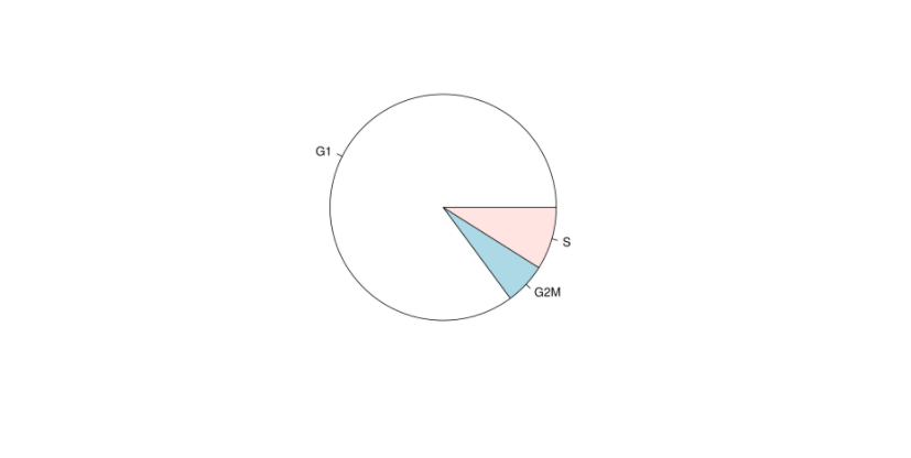

6. Plot QC

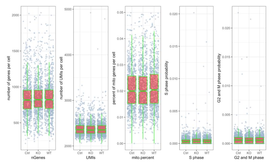
默認(rèn)情況下的繪圖功能都將創(chuàng)建交互式html文件，可以設(shè)置interactive = FALSE來(lái)關(guān)閉。

# 繪制 三個(gè)分組中UMIs, genes和 percent mito的beanplot分布圖，想單獨(dú)畫地話可以用`?stats.plot`help一下如何修改參數(shù)
stats.plot(my.obj,
    plot.type = "all.in.one",
    out.name = "UMI-plot",
    interactive = FALSE,
    cell.color = "slategray3",
    cell.size = 1,
    cell.transparency = 0.5,
    box.color = "red",
    box.line.col = "green")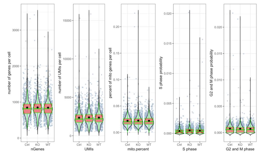

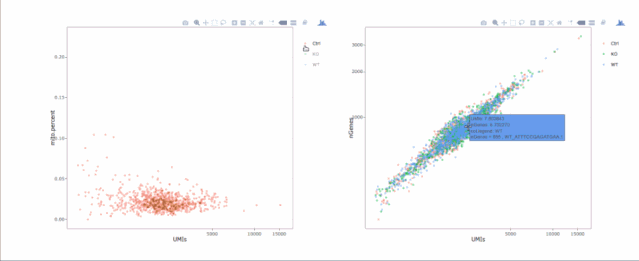
# 繪制散點(diǎn)圖查看線粒體基因和基因分布，注意參數(shù)`plot.type`
stats.plot(my.obj, plot.type = "point.mito.umi", out.name = "mito-umi-plot")###該圖為線粒體基因和UMI的相關(guān)表達(dá)分布（一般原則下會(huì)認(rèn)為線粒體基因比例較高可能為破碎衰老細(xì)胞，可以設(shè)置cutoff值去掉，但如果研究為高代謝或本身耗能較多的細(xì)胞時(shí)需要考慮）
stats.plot(my.obj, plot.type = "point.gene.umi", out.name = "gene-umi-plot")###此圖為UMI和GENE的表達(dá)分布（原則上遵循線性分布）

R語(yǔ)言 - 散點(diǎn)圖繪制

7. 過(guò)濾細(xì)胞

my.obj <- cell.filter(my.obj,
    min.mito = 0,
    max.mito = 0.05,
    min.genes = 200,
    max.genes = 2400,
    min.umis = 0,
    max.umis = Inf)

#[1] "cells with min mito ratio of 0 and max mito ratio of 0.05 were filtered." 保留線粒體基因比例在0到0.05的細(xì)胞
#[1] "cells with min genes of 200 and max genes of 2400 were filtered." 保留基因數(shù)在200到2400之間的細(xì)胞
#[1] "No UMI number filter" 不通過(guò)UMI數(shù)和細(xì)胞ID來(lái)篩選
#[1] "No cell filter by provided gene/genes"
#[1] "No cell id filter"
#[1] "filters_set.txt file has beed generated and includes the filters set for this experiment."篩選之后會(huì)生成一個(gè)文件filter_set，含有實(shí)驗(yàn)的篩選設(shè)置
# more examples 也可以通過(guò)基因和細(xì)胞ID來(lái)篩選
# my.obj <- cell.filter(my.obj, filter.by.gene = c("RPL13","RPL10")) # filter our cell having no counts for these genes
# my.obj <- cell.filter(my.obj, filter.by.cell.id = c("WT_AAACATACAACCAC.1")) # filter our cell cell by their cell ids.

# 查看剩下的細(xì)胞數(shù)(線粒體基因比例在0到0.05,基因數(shù)在200到2400之間)
dim([email protected])
#[1] 32738  2637
# 過(guò)濾掉了63個(gè)細(xì)胞

• Hemberg-lab單細(xì)胞轉(zhuǎn)錄組數(shù)據(jù)分析（九）- Scater包單細(xì)胞過(guò)濾

• Hemberg-lab單細(xì)胞轉(zhuǎn)錄組數(shù)據(jù)分析（十）- Scater基因評(píng)估和過(guò)濾

8. 進(jìn)行標(biāo)準(zhǔn)化

可以根據(jù)自己的研究對(duì)數(shù)據(jù)進(jìn)行標(biāo)準(zhǔn)化。還可以使用iCellR以外的工具對(duì)數(shù)據(jù)進(jìn)行標(biāo)準(zhǔn)化，并將數(shù)據(jù)導(dǎo)入iCellR。對(duì)于大多數(shù)單細(xì)胞研究，建議使用“ranked.glsf”標(biāo)準(zhǔn)化。這種標(biāo)準(zhǔn)化化比較適合具有大量零的矩陣。且在合并數(shù)據(jù)（操作參考步驟2：匯總數(shù)據(jù)）的情況下，也能對(duì)批次進(jìn)行校正。

my.obj <- norm.data(my.obj,
     norm.method = "ranked.glsf",
     top.rank = 500) # best for scRNA-Seq
# **更多的標(biāo)準(zhǔn)化方式**
#my.obj <- norm.data(my.obj, norm.method = "ranked.deseq", top.rank = 500)
#my.obj <- norm.data(my.obj, norm.method = "deseq") # best for bulk RNA-Seq
#my.obj <- norm.data(my.obj, norm.method = "global.glsf") # best for bulk RNA-Seq
#my.obj <- norm.data(my.obj, norm.method = "rpm", rpm.factor = 100000) # best for bulk RNA-Seq
#my.obj <- norm.data(my.obj, norm.method = "spike.in", spike.in.factors = NULL)
#my.obj <- norm.data(my.obj, norm.method = "no.norm") # if the data is already normalized

9. 進(jìn)行二次QC

my.obj <- qc.stats(my.obj,which.data = "main.data")
### 該次QC的主要目的就是計(jì)算UMI數(shù)量，每個(gè)細(xì)胞的基因以及每個(gè)細(xì)胞和細(xì)胞周期基因的線粒體基因的百分比。從圖中可以看出其細(xì)胞周期相關(guān)基因表達(dá)較低，線粒體基因表達(dá)比例也較低
stats.plot(my.obj,
    plot.type = "all.in.one",
    out.name = "UMI-plot",
    interactive = F,
    cell.color = "slategray3",
    cell.size = 1,
    cell.transparency = 0.5,
    box.color = "red",
    box.line.col = "green",
    back.col = "white")

R語(yǔ)言 - 箱線圖（小提琴圖、抖動(dòng)圖、區(qū)域散點(diǎn)圖）

10. Scale data

my.obj <- data.scale(my.obj)  # 對(duì)數(shù)據(jù)進(jìn)行中心化和標(biāo)準(zhǔn)化處理

11.進(jìn)行g(shù)ene統(tǒng)計(jì)

my.obj <- gene.stats(my.obj, which.data = "main.data")
head([email protected][order([email protected]$numberOfCells, decreasing = T),])  # 將數(shù)據(jù)通過(guò)擁有該基因的細(xì)胞數(shù)按從大到小進(jìn)行排序
#       genes numberOfCells totalNumberOfCells percentOfCells  meanExp
#30303 TMSB4X          2637               2637      100.00000 38.55948
#3633     B2M          2636               2637       99.96208 45.07327
#14403 MALAT1          2636               2637       99.96208 70.95452
#27191 RPL13A          2635               2637       99.92416 32.29009
#27185  RPL10          2632               2637       99.81039 35.43002
#27190  RPL13          2630               2637       99.73455 32.32106
#               SDs condition
#30303 7.545968e-15       all
#3633  2.893940e+01       all
#14403 7.996407e+01       all
#27191 2.783799e+01       all
#27185 2.599067e+01       all
#27190 2.661361e+01       all

12.制作聚類的基因模型

在bulk RNA-seq數(shù)據(jù)中，用平均表達(dá)值meanExp排名前500的基因(設(shè)置參數(shù)base.mean.rank對(duì)樣本進(jìn)行聚類是非常常見(jiàn)的，主要原因是為了降低噪聲。在scRNA-seq數(shù)據(jù)中也可以這樣做。并加上ranked.glsf歸一化，會(huì)較為擅長(zhǎng)處理具有大量零的矩陣。

# 看一下高變基因集
make.gene.model(my.obj, my.out.put = "plot",
    dispersion.limit = 1.5,
    base.mean.rank = 500,
    no.mito.model = T,
    mark.mito = T,
    interactive = F,
    no.cell.cycle = T,
    out.name = "gene.model")

# 將高變基因集注入`my.obj` 中
my.obj <- make.gene.model(my.obj, my.out.put = "data",
    dispersion.limit = 1.5,
    base.mean.rank = 500,
    no.mito.model = T,
    mark.mito = T,
    interactive = F,
    no.cell.cycle = T,
    out.name = "gene.model")
head([email protected])  # 高變基因
# "ACTB"  "ACTG1" "ACTR3" "AES"   "AIF1"  "ALDOA"
# get html plot (optional)
#make.gene.model(my.obj, my.out.put = "plot",
#    dispersion.limit = 1.5,
#    base.mean.rank = 500,
#    no.mito.model = T,
#    mark.mito = T,
#    interactive = T,
#    out.name = "plot4_gene.model")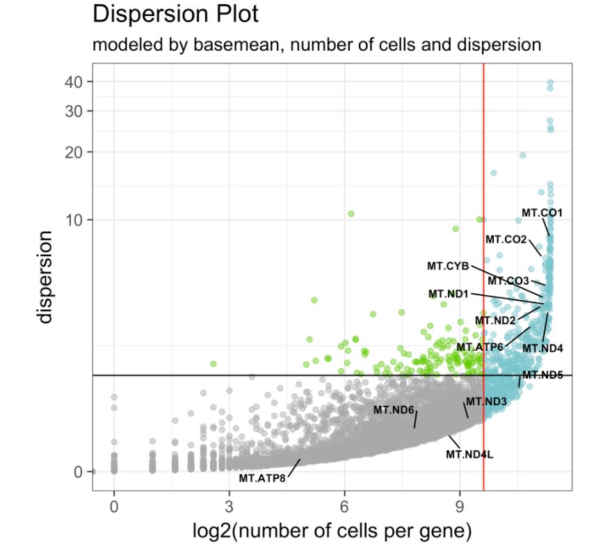

13. 進(jìn)行降維

降維是為了在信息損失較少的情況下，以比原始特征數(shù)量少得多的特征（基因）來(lái)表示數(shù)據(jù)，更好地捕捉細(xì)胞之間的關(guān)系，常見(jiàn)降維的方法有PCA，t-SNE，umap和diffusion map。（Hemberg-lab單細(xì)胞轉(zhuǎn)錄組數(shù)據(jù)分析（十一）- Scater單細(xì)胞表達(dá)譜PCA可視化）

PCA分析

my.obj <- run.pca(my.obj, method = "gene.model", gene.list = [email protected],data.type = "main",batch.norm = F)
opt.pcs.plot(my.obj)
##下圖為典型的滾石圖，當(dāng)趨勢(shì)越趨于平緩表明其PC值作用越小，下圖PCA取到10。這一步是可選的，可能在一些情況下也是不適用的。# 2 round PCA (to find top genes in the first 10 PCs and re-run PCA for better clustering
## This is optional and might not be good in some cases
length([email protected])
# 585
my.obj <- find.dim.genes(my.obj, dims = 1:10,top.pos = 20, top.neg = 20) # (optional)
length([email protected])
# 208
# second round PC
my.obj <- run.pca(my.obj, method = "gene.model", gene.list = [email protected],data.type = "main",batch.norm = F)
[email protected]

Hemberg-lab單細(xì)胞轉(zhuǎn)錄組數(shù)據(jù)分析（十一）- Scater單細(xì)胞表達(dá)譜PCA可視化

更多降維方法

# tSNE
my.obj <- run.pc.tsne(my.obj, dims = 1:10)
# UMAP
my.obj <- run.umap(my.obj, dims = 1:10, method = "naive")
# or
# my.obj <- run.umap(my.obj, dims = 1:10, method = "umap-learn")
# diffusion map
# this requires python packge phate
# pip install --user phate
# Install phateR version 2.9
# wget https://cran.r-project.org/src/contrib/Archive/phateR/phateR_0.2.9.tar.gz
# install.packages('phateR/', repos = NULL, type="source")
library(phateR)
my.obj <- run.diffusion.map(my.obj, dims = 1:10, method = "phate")

14. 對(duì)細(xì)胞進(jìn)行聚類分析

“聚類是針對(duì)給定的樣本，依據(jù)它們特征的相似度或距離，將其歸并到若干個(gè)“類”或“簇”的數(shù)據(jù)分析問(wèn)題。一個(gè)類是樣本的一個(gè)子集。直觀上，相似的樣本聚集在相同的類，不相似的樣本分散在不同的類。這里，樣本之間的相似度或距離起著重要作用。”
降維是對(duì)feature (gene) 進(jìn)行操作，而聚類是對(duì)sample進(jìn)行操作，建議在得到高變基因以及降維后操作。(基因表達(dá)聚類分析之初探SOM)

建議使用以下默認(rèn)選項(xiàng)：

my.obj <- run.clustering(my.obj,
    clust.method = "kmeans",     # 聚類方式為k-means
    dist.method = "euclidean",   # 距離計(jì)算是歐氏距離，有非常明確的空間距離概念
    index.method = "silhouette",
    max.clust = 25,
    min.clust = 2,
    dims = 1:10)

# 如果要手動(dòng)設(shè)置cluster數(shù)量，而不使用預(yù)測(cè)的最佳數(shù)量，請(qǐng)將最小值和最大值設(shè)置為所需的數(shù)量:
#my.obj <- run.clustering(my.obj,
#    clust.method = "ward.D",
#    dist.method = "euclidean",
#    index.method = "ccc",
#    max.clust = 8,
#    min.clust = 8,
#    dims = 1:10)
# more examples
#my.obj <- run.clustering(my.obj,
#    clust.method = "ward.D",
#    dist.method = "euclidean",
#    index.method = "kl",
#    max.clust = 25,
#    min.clust = 2,
#    dims = 1:10)

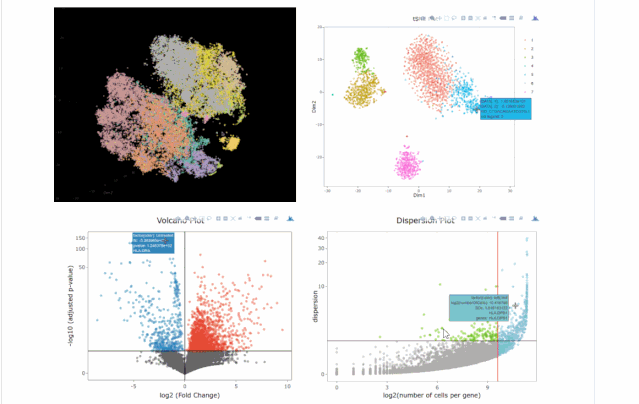
15. 數(shù)據(jù)可視化

# clusters
A= cluster.plot(my.obj,plot.type = "pca",interactive = F)
B= cluster.plot(my.obj,plot.type = "umap",interactive = F)
C= cluster.plot(my.obj,plot.type = "tsne",interactive = F)
D= cluster.plot(my.obj,plot.type = "diffusion",interactive = F)
#下圖通過(guò)不同降維方式進(jìn)行展示，其實(shí)我們可以看出，在該組數(shù)據(jù)中還是t-sne降維后的可視化表達(dá)方式最好（細(xì)胞之間的分離度較好）
library(gridExtra)
grid.arrange(A,B,C,D)
# conditions
A= cluster.plot(my.obj,plot.type = "pca",col.by = "conditions",interactive = F)
B= cluster.plot(my.obj,plot.type = "umap",col.by = "conditions",interactive = F)
C= cluster.plot(my.obj,plot.type = "tsne",col.by = "conditions",interactive = F)
D= cluster.plot(my.obj,plot.type = "diffusion",col.by = "conditions",interactive = F)
#在下圖中我們可以發(fā)現(xiàn)無(wú)論哪種降維方式均沒(méi)有batch effect不同條件下的細(xì)胞重合度較好；library(gridExtra)
grid.arrange(A,B,C,D)

16. 三維圖，密度圖和交互式圖

# 2D展示
cluster.plot(my.obj,
    cell.size = 1,
    plot.type = "tsne",
    cell.color = "black",
    back.col = "white",
    col.by = "clusters",
    cell.transparency = 0.5,
    clust.dim = 2,
    interactive = F)

# 可交互的2D圖
cluster.plot(my.obj,
    plot.type = "tsne",
    col.by = "clusters",
    clust.dim = 2,
    interactive = T,
    out.name = "tSNE_2D_clusters")
# 可交互的3D圖
cluster.plot(my.obj,
    plot.type = "tsne",
    col.by = "clusters",
    clust.dim = 3,
    interactive = T,
    out.name = "tSNE_3D_clusters")
# cluster的密度圖
cluster.plot(my.obj,
    plot.type = "pca",
    col.by = "clusters",
    interactive = F,
    density=T)
# Density plot for conditions
cluster.plot(my.obj,
    plot.type = "pca",
    col.by = "conditions",
    interactive = F,
    density=T)
#下圖為不同可視化方式，盡管方法多種多樣，但個(gè)人感覺(jué)還是2D的方式展示是最為合適的。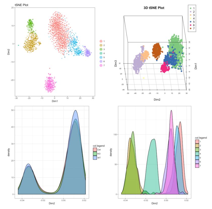

17. 不同cluster和條件下細(xì)胞比例

#如果normalize.ncell = TRUE，它將在三種狀態(tài)（conditions）隨機(jī)**降采樣（down sample）**，因此所有條件都具有相同數(shù)量的細(xì)胞，如果為FALSE則輸出原始細(xì)胞數(shù)。#下圖分別是在不同條件下細(xì)胞的比例關(guān)系，KO，WT，ctrl都是我們較為常見(jiàn)的細(xì)胞分組。# bar plot
clust.cond.info(my.obj, plot.type = "bar", normalize.ncell = FALSE, my.out.put = "plot")
# Pie chart
clust.cond.info(my.obj, plot.type = "pie", normalize.ncell = FALSE, ,my.out.put = "plot")
# data
my.obj <- clust.cond.info(my.obj, plot.type = "bar", normalize.ncell = F)
#head([email protected])
#  conditions clusters Freq
#1       ctrl        1  199
#2         KO        1  170
#3         WT        1  182
#4       ctrl        2  106
#5         KO        2  116
#6         WT        2  113

到這里，我們其實(shí)已經(jīng)表現(xiàn)了許多的plot，下期接著介紹吧！

單細(xì)胞

• 收藏 北大生信平臺(tái)” 單細(xì)胞分析、染色質(zhì)分析” 視頻和PPT分享

• Science: 小鼠腎臟單細(xì)胞轉(zhuǎn)錄組+突變分析揭示腎病潛在的細(xì)胞靶標(biāo)

• Science：通過(guò)單細(xì)胞轉(zhuǎn)錄組測(cè)序揭示玉米減數(shù)分裂進(jìn)程 | 很好的單細(xì)胞分析案例

• Nature 首次對(duì)阿爾茨海默病進(jìn)行單細(xì)胞轉(zhuǎn)錄組分析|詳細(xì)解讀

• Cell 深度 一套普遍適用于各類單細(xì)胞測(cè)序數(shù)據(jù)集的錨定整合方案

• 骨髓基質(zhì)在正常和白血病個(gè)體中的細(xì)胞圖譜 Cell,Nature聯(lián)袂解析

• 癌中之王：基質(zhì)微環(huán)境塑造胰腺癌瘤內(nèi)結(jié)構(gòu)|Cell

• Nature系列 整合單細(xì)胞轉(zhuǎn)錄組學(xué)和質(zhì)譜流式確定類風(fēng)濕性關(guān)節(jié)炎滑膜組織中的炎癥細(xì)胞狀態(tài) 詳細(xì)解讀

• 單細(xì)胞轉(zhuǎn)錄組教程匯總
  

• 10X單細(xì)胞測(cè)序分析軟件:Cell ranger，從拆庫(kù)到定量

• Hemberg-lab單細(xì)胞轉(zhuǎn)錄組數(shù)據(jù)分析（一）- 引言

• Hemberg-lab單細(xì)胞轉(zhuǎn)錄組數(shù)據(jù)分析（二）- 實(shí)驗(yàn)平臺(tái)

• Hemberg-lab單細(xì)胞轉(zhuǎn)錄組數(shù)據(jù)分析（三）- 原始數(shù)據(jù)質(zhì)控

• Hemberg-lab單細(xì)胞轉(zhuǎn)錄組數(shù)據(jù)分析（四）- 文庫(kù)拆分和細(xì)胞鑒定

• Hemberg-lab單細(xì)胞轉(zhuǎn)錄組數(shù)據(jù)分析（五）- STAR, Kallisto定量

• Hemberg-lab單細(xì)胞轉(zhuǎn)錄組數(shù)據(jù)分析（六）- 構(gòu)建表達(dá)矩陣，UMI介紹

• Hemberg-lab單細(xì)胞轉(zhuǎn)錄組數(shù)據(jù)分析（七）- 導(dǎo)入10X和SmartSeq2數(shù)據(jù)Tabula Muris

• Hemberg-lab單細(xì)胞轉(zhuǎn)錄組數(shù)據(jù)分析（八）- Scater包輸入導(dǎo)入和存儲(chǔ)

• Hemberg-lab單細(xì)胞轉(zhuǎn)錄組數(shù)據(jù)分析（九）- Scater包單細(xì)胞過(guò)濾

• Hemberg-lab單細(xì)胞轉(zhuǎn)錄組數(shù)據(jù)分析（十）- Scater基因評(píng)估和過(guò)濾

• Hemberg-lab單細(xì)胞轉(zhuǎn)錄組數(shù)據(jù)分析（十一）- Scater單細(xì)胞表達(dá)譜PCA可視化

• Hemberg-lab單細(xì)胞轉(zhuǎn)錄組數(shù)據(jù)分析（十二）- Scater單細(xì)胞表達(dá)譜tSNE可視化

• 如何火眼金睛鑒定那些單細(xì)胞轉(zhuǎn)錄組中的混雜因素

• 什么？你做的差異基因方法不合適？

• 單細(xì)胞分群后，怎么找到Marker基因定義每一類群？

• 在線平臺(tái)如何做單細(xì)胞測(cè)序分析全套？有它so easy!

• 植物單細(xì)胞轉(zhuǎn)錄組的春天來(lái)了，還不上車？Science, PC, PP, MP, bioRxiv各一個(gè)

• 三人成虎，概率卻不足十分之五？

• 一文掌握GSEA，超詳細(xì)教程

• 這個(gè)只需一步就可做富集分析的網(wǎng)站還未發(fā)表就被CNS等引用超過(guò)350次

• 什么，你算出的P-value看上去像齊天大圣變的廟？

• GO、GSEA富集分析一網(wǎng)打進(jìn)

• GSEA富集分析 - 界面操作

• 無(wú)需寫代碼的高顏值富集分析神器

• 去東方，最好用的在線GO富集分析工具

• 跨物種單細(xì)胞分析發(fā)現(xiàn)胰腺導(dǎo)管癌中一類有免疫原性的抗原呈遞成纖維細(xì)胞

• NCB|心咽發(fā)育多樣化的單細(xì)胞轉(zhuǎn)錄軌跡分析

• 七龍珠|召喚一份單細(xì)胞數(shù)據(jù)庫(kù)匯總

• 用了這么多年的PCA可視化竟然是錯(cuò)的！！！

• 單細(xì)胞預(yù)測(cè)Doublets軟件包匯總-過(guò)渡態(tài)細(xì)胞是真的嗎？

• Seurat亮點(diǎn)之細(xì)胞周期評(píng)分和回歸

• cellassign：用于腫瘤微環(huán)境分析的單細(xì)胞注釋工具（9月Nature）

• Nature重磅綜述 |關(guān)于RNA-seq，你想知道的都在這

高顏值免費(fèi)在線繪圖

往期精品(點(diǎn)擊圖片直達(dá)文字對(duì)應(yīng)教程)

機(jī)器學(xué)習(xí)

后臺(tái)回復(fù)“生信寶典福利第一波”或點(diǎn)擊閱讀原文獲取教程合集