
數(shù)據(jù)特征分析技能——統(tǒng)計分析
統(tǒng)計指標對定量數(shù)據(jù)進行統(tǒng)計描述,常從集中趨勢和離中趨勢兩個方面進行分析
import numpy as np
import pandas as pd
import matplotlib.pyplot as plt
% matplotlib inline
1
2
3
4
集中趨勢度量
指一組數(shù)據(jù)向某一中心靠攏的傾向,核心在于尋找數(shù)據(jù)的代表值或中心值
取得集中趨勢代表值的方法有兩種:數(shù)值平均數(shù)和位置平均數(shù)?
- 數(shù)值平均數(shù)?
- 算數(shù)平均數(shù)?
- 調(diào)和平均數(shù)?
- 幾何平均數(shù)?
- 位置平均數(shù)?
- 眾數(shù)?
- 中位數(shù)
數(shù)值平均數(shù)
算數(shù)平均數(shù)
關注數(shù)值,魯棒性弱(穩(wěn)定性較弱,易受到異常值影響)
data = pd.DataFrame({'value':np.random.randint(100,120,100),
                    'f':np.random.rand(100)})
data['f'] = data['f'] / data['f'].sum()  # f為權(quán)重,這里將f列設置成總和為1的權(quán)重占比
print(data.head())
print('-----------------')

# 算數(shù)平均值
mean = data['value'].mean()
print('算數(shù)平均數(shù)為:%.2f'%mean)

mean_w = (data['value'] * data['f']).sum() / data['f'].sum()
print('加權(quán)算數(shù)平均值為:%.2f'%mean_w)
# 加權(quán)算數(shù)平均值 = (x1f1 + x2f2 + ... + xnfn) / (f1 + f2 + ... + fn)
1
2
3
4
5
6
7
8
9
10
11
12
13
          f  value
0  0.014970    118
1  0.007184    116
2  0.007459    101
3  0.005892    110
4  0.016599    119
-----------------
算數(shù)平均數(shù)為:110.09
加權(quán)算數(shù)平均值為:110.69
1
2
3
4
5
6
7
8
9
幾何平均數(shù)
計算幾何平均數(shù)要求各觀察值之間存在連乘積關系,它的主要用途是?
1. 對比率、指數(shù)等進行平均?
2. 計算平均發(fā)展速度?
- 樣本數(shù)據(jù)非負,主要用于對數(shù)正態(tài)分布?
3. 復利下的平均年利率?
4. 連續(xù)作業(yè)的車間求產(chǎn)品的平均合格率
幾何平均數(shù)
# 一位投資者持有股票,1996年,1997年,1998年,1999年收益率分別為
# 4.5%, 2.0%, 3.5%, 5.4%,
# 求此4年內(nèi)平均收益率
from scipy.stats import gmean
data_g = gmean(data['value'])
data_g
1
2
3
4
5
6
109.96165465844449
1
位置平均數(shù)
中位數(shù):?
- 關注順序,魯棒性強眾數(shù):?
- 關注頻次
# 中位數(shù)
med = data['value'].median()
print('中位數(shù)為%i' % med)
# 中位數(shù)指將總體各單位標志按照大小順序排列后,中間位置的數(shù)字


# 眾數(shù)
m = data['value'].mode()
print('眾數(shù)為',m.tolist())
# 眾數(shù)是一組數(shù)據(jù)中出現(xiàn)次數(shù)最多的數(shù),這里可能返回多個值


# 密度曲線
data['value'].plot(kind='kde',style='--k',grid=True,figsize=(10,6))


# 簡單算術(shù)平均
plt.axvline(mean,hold=None,color='r',linestyle='--',alpha=0.8)
plt.text(mean+5,0.005,'簡單算術(shù)平均值:%.2f' % mean,color='r',fontsize=15)


# 加權(quán)平均數(shù)
plt.axvline(mean_w,hold=None,color='b',linestyle='--',alpha=0.8)
plt.text(mean+5,0.01,'加權(quán)平均值:%.2f' % mean_w,color='b',fontsize=15)

# 幾何平均數(shù)
plt.axvline(data_g,hold=None,color='g',linestyle='--',alpha=0.8)
plt.text(mean+5,0.015,'幾何平均值:%.2f' % data_g,color='g',fontsize=15)

# 中位數(shù)
plt.axvline(med,hold=None,color='y',linestyle='--',alpha=0.8)
plt.text(mean+5,0.020,'幾何平均值:%.2f' % med,color='y',fontsize=15)
1
2
3
4
5
6
7
8
9
10
11
12
13
14
15
16
17
18
19
20
21
22
23
24
25
26
27
28
29
30
31
32
33
中位數(shù)為110
眾數(shù)為 [108]
1
2

離中趨勢度
是指一組數(shù)據(jù)中個數(shù)據(jù)值以不同程度偏離其中心(平均數(shù))的趨勢,又稱標志變動度
# 創(chuàng)建數(shù)據(jù),銷售數(shù)據(jù)
data = pd.DataFrame({'A_sale':np.random.rand(30)*1000,
                    'B_sale':np.random.rand(30)*1000},
                   index = pd.period_range('20170601','20170630'))
print(data.head())
1
2
3
4
5
                A_sale      B_sale
2017-06-01  574.693080  970.059264
2017-06-02  278.487440  683.602258
2017-06-03  830.472896  293.102768
2017-06-04  505.211093  268.009253
2017-06-05  316.383594  134.011541
1
2
3
4
5
6
極差與分位差
極差:?
- 沒有考慮中間值的變動情況,測定離中趨勢時不準確分位差:?
- 從一組數(shù)據(jù)踢出部分極端值后的從新計算類似極差的指標,常用的有四分位差,八分位差
a_r = data['A_sale'].max() - data['A_sale'].min()
b_r = data['B_sale'].max() - data['B_sale'].min()
print('A產(chǎn)品銷售額極差為:%.2f,B產(chǎn)品銷售額極差為:%.2f'%(a_r,b_r))
1
2
3
A產(chǎn)品銷售額極差為:920.98,B產(chǎn)品銷售額極差為:914.30
1
sta = data['A_sale'].describe()
stb = data['B_sale'].describe()
#print(sta)
a_iqr = sta.loc['75%'] - sta.loc['25%']
b_iqr = stb.loc['75%'] - stb.loc['25%']
print('A銷售額的分位差為:%.2f, B銷售額的分位差為:%.2f' % (a_iqr,b_iqr))
1
2
3
4
5
6
A銷售額的分位差為:481.57, B銷售額的分位差為:508.45
1
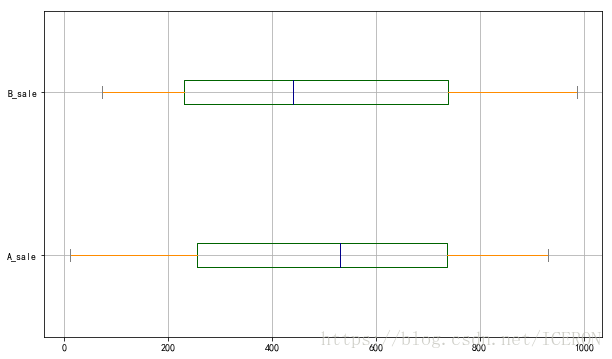
# 繪制箱型圖

color = dict(boxes='DarkGreen', whiskers='DarkOrange', medians='DarkBlue', caps='Gray')
data.plot.box(vert=False,grid = True,color = color,figsize = (10,6))
# 箱型圖
1
2
3
4
5
方差與標準差
平均差:平均差是總體所有單位與其算術(shù)平均數(shù)的離差絕對值的算術(shù)平均數(shù),1范數(shù),異常值影響?
M D = ∑ N ‖ x ? x ˉ ‖ N 方差:差的平方的均值,2范數(shù),異常值影響
總體方差?
樣本方差?
標準差:方差的算數(shù)平方根(應用最廣)
平均差 VS 方差:對異常值的敏感程度不同
離散系數(shù)(常用的是標準差系數(shù):數(shù)據(jù)標準差和算數(shù)平均數(shù)的比)
a_std = sta.loc['std']
b_std = stb.loc['std']
a_var = data['A_sale'].var()
b_var = data['B_sale'].var()
print('A銷售額的標準差為:%.2f, B銷售額的標準差為:%.2f' % (a_std,b_std))
print('A銷售額的方差為:%.2f, B銷售額的方差為:%.2f' % (a_var,b_var))
# 方差 → 各組中數(shù)值與算數(shù)平均數(shù)離差平方的算術(shù)平均數(shù)
# 標準差 → 方差的平方根
# 標準差是最常用的離中趨勢指標 → 標準差越大,離中趨勢越明顯
1
2
3
4
5
6
7
8
9
A銷售額的標準差為:292.12, B銷售額的標準差為:293.35
A銷售額的方差為:85331.19, B銷售額的方差為:86052.83
1
2
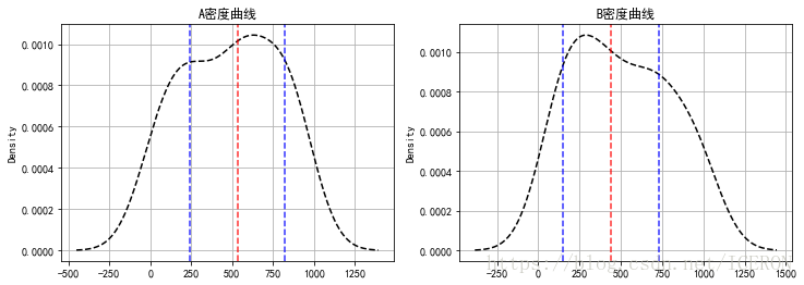
fig = plt.figure(figsize = (12,4))
ax1 = fig.add_subplot(1,2,1)
data['A_sale'].plot(kind = 'kde',style = 'k--',grid = True,title = 'A密度曲線')
plt.axvline(sta.loc['50%'],hold=None,color='r',linestyle="--",alpha=0.8)
plt.axvline(sta.loc['50%'] - a_std,hold=None,color='b',linestyle="--",alpha=0.8)
plt.axvline(sta.loc['50%'] + a_std,hold=None,color='b',linestyle="--",alpha=0.8)
# A密度曲線,1個標準差

ax2 = fig.add_subplot(1,2,2)
data['B_sale'].plot(kind = 'kde',style = 'k--',grid = True,title = 'B密度曲線')
plt.axvline(stb.loc['50%'],hold=None,color='r',linestyle="--",alpha=0.8)
plt.axvline(stb.loc['50%'] - b_std,hold=None,color='b',linestyle="--",alpha=0.8)
plt.axvline(stb.loc['50%'] + b_std,hold=None,color='b',linestyle="--",alpha=0.8)
# B密度曲線,1個標準差
1
2
3
4
5
6
7
8
9
10
11
12
13
14
推薦閱讀
《數(shù)據(jù)科學與人工智能》公眾號推薦朋友們學習和使用Python語言,需要加入Python語言群的,請掃碼加我個人微信,備注【姓名-Python群】,我誠邀你入群,大家學習和分享。