【數(shù)據(jù)競賽】從0梳理1場數(shù)據(jù)挖掘賽事！

賽事分析

1. 本次賽題為數(shù)據(jù)挖掘類型，通過機(jī)器學(xué)習(xí)算法進(jìn)行建模預(yù)測。
2. 是一個(gè)典型的回歸問題。
3. 主要應(yīng)用xgb、lgb、catboost，以及pandas、numpy、matplotlib、seabon、sklearn、keras等數(shù)據(jù)挖掘常用庫或者框架來進(jìn)行數(shù)據(jù)挖掘任務(wù)。
4. 通過EDA來挖掘數(shù)據(jù)的信息。
5. 賽事地址（復(fù)制打開或閱讀原文）：https://tianchi.aliyun.com/s/f4ea3bec4429458ea03ef461cda87c3f
   
   
   

數(shù)據(jù)概況

了解列的性質(zhì)會有助于我們對于數(shù)據(jù)的理解和后續(xù)分析。Tip:匿名特征，就是未告知數(shù)據(jù)列所屬的性質(zhì)的特征列。數(shù)據(jù)下載地址：https://tianchi.aliyun.com/competition/entrance/531858/information

代碼實(shí)踐

Step 1:環(huán)境準(zhǔn)備（導(dǎo)入相關(guān)庫）

## 基礎(chǔ)工具
import numpy as np
import pandas as pd
import warnings
import matplotlib
import matplotlib.pyplot as plt
import seaborn as sns
from scipy.special import jn
from IPython.display import display, clear_output
import time

warnings.filterwarnings('ignore')
%matplotlib inline

## 數(shù)據(jù)處理
from sklearn import preprocessing

## 數(shù)據(jù)降維處理的
from sklearn.decomposition import PCA,FastICA,FactorAnalysis,SparsePCA

## 模型預(yù)測的
import lightgbm as lgb
import xgboost as xgb

## 參數(shù)搜索和評價(jià)的
from sklearn.model_selection import GridSearchCV,cross_val_score,StratifiedKFold,train_test_split
from sklearn.metrics import mean_squared_error, mean_absolute_error

Step 2:數(shù)據(jù)讀取

## 通過Pandas對于數(shù)據(jù)進(jìn)行讀取 (pandas是一個(gè)很友好的數(shù)據(jù)讀取函數(shù)庫)
#Train_data = pd.read_csv('datalab/231784/used_car_train_20200313.csv', sep=' ')
#TestA_data = pd.read_csv('datalab/231784/used_car_testA_20200313.csv', sep=' ')

path = './data/'
## 1) 載入訓(xùn)練集和測試集；
Train_data = pd.read_csv(path+'train.csv', sep=' ')
TestA_data = pd.read_csv(path+'testA.csv', sep=' ')

## 輸出數(shù)據(jù)的大小信息
print('Train data shape:',Train_data.shape)
print('TestA data shape:',TestA_data.shape)

Train data shape: (150000, 31)
TestA data shape: (50000, 30)

可以發(fā)現(xiàn)訓(xùn)練集有 15w 樣本，而測試集有 5w 樣本，特征維度并非很高，總體只有30維。

1) 數(shù)據(jù)簡要瀏覽

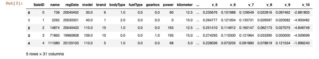
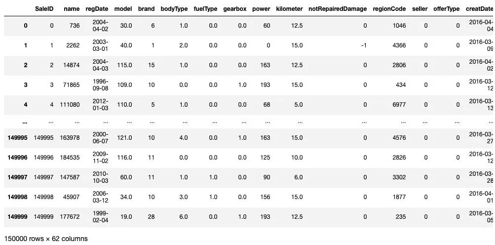
## 通過.head() 簡要瀏覽讀取數(shù)據(jù)的形式
Train_data.head()

2) 數(shù)據(jù)信息查看

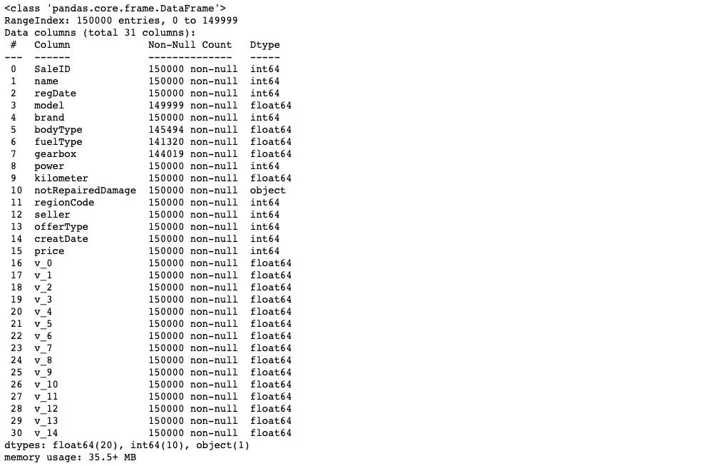
## 通過 .info() 簡要可以看到對應(yīng)一些數(shù)據(jù)列名，以及NAN缺失信息
Train_data.info()

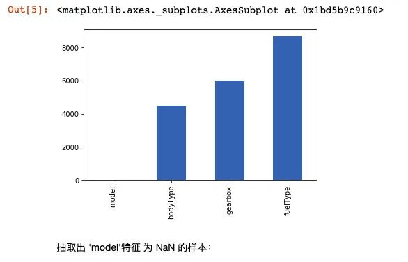
# nan可視化
missing = Train_data.isnull().sum()
missing = missing[missing > 0]
missing.sort_values(inplace=True)
missing.plot.bar()

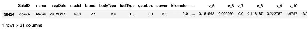
抽取出 'model'特征 為 NaN 的樣本：

Train_data[np.isnan(Train_data['model'])]

TestA_data.info()

通過對于數(shù)據(jù)的基礎(chǔ) Infomation的查看，我們知道 'model','bodyType','fuelType','gearbox'特征 中存在缺失。

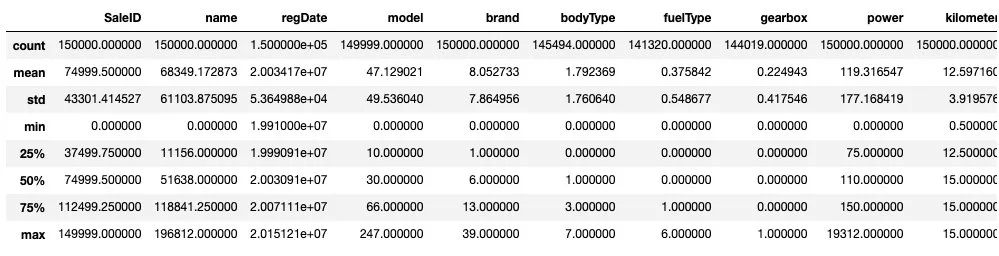
3) 數(shù)據(jù)統(tǒng)計(jì)信息瀏覽

#顯示所有列
pd.set_option('display.max_columns', None)

## 通過 .describe() 可以查看數(shù)值特征列的一些統(tǒng)計(jì)信息
Train_data.describe()

TestA_data.describe()

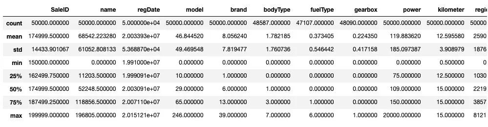
通過數(shù)據(jù)的統(tǒng)計(jì)信息，可以對于數(shù)據(jù)中的特征的變化情況有一個(gè)整體的了解。

Step 3: 數(shù)據(jù)分析（EDA）

1) 提取數(shù)值類型特征列名

numerical_cols = Train_data.select_dtypes(exclude = 'object').columns
print(numerical_cols)

categorical_cols = Train_data.select_dtypes(include = 'object').columns
print(categorical_cols)

# out: Index(['notRepairedDamage'], dtype='object')

首先我們對于非數(shù)字特征列進(jìn)行數(shù)值化處理

set(Train_data['notRepairedDamage'])

# Out：{'-', '0.0', '1.0'}

Train_data['notRepairedDamage'] = Train_data['notRepairedDamage'].map({'-':-1,'0.0':0,'1.0':1})
TestA_data['notRepairedDamage'] = TestA_data['notRepairedDamage'].map({'-':-1,'0.0':0,'1.0':1})

由于數(shù)據(jù)特征可以分為 三種不同類型的特征，分別為時(shí)間特征，類別特征 和 數(shù)值類型特征, 我們對于不同特征進(jìn)行分類別處理。

date_features = ['regDate', 'creatDate']
numeric_features = ['power', 'kilometer'] + ['v_{}'.format(i) for i in range(15)]
categorical_features = ['name', 'model', 'brand', 'bodyType', 'fuelType', 'gearbox', 'notRepairedDamage', 'regionCode',]

首先對于時(shí)間特征進(jìn)行處理:

from tqdm import tqdm

def date_proc(x):
    m = int(x[4:6])
    if m == 0:
        m = 1
    return x[:4] + '-' + str(m) + '-' + x[6:]

def num_to_date(df,date_cols):
    for f in tqdm(date_cols):
        df[f] = pd.to_datetime(df[f].astype('str').apply(date_proc))
        df[f + '_year'] = df[f].dt.year
        df[f + '_month'] = df[f].dt.month
        df[f + '_day'] = df[f].dt.day
        df[f + '_dayofweek'] = df[f].dt.dayofweek
    return df

Train_data = num_to_date(Train_data,date_features)
TestA_data = num_to_date(TestA_data,date_features)

plt.figure()
plt.figure(figsize=(16, 6))
i = 1
for f in date_features:
    for col in ['year', 'month', 'day', 'dayofweek']:
        plt.subplot(2, 4, i)
        i += 1
        v = Train_data[f + '_' + col].value_counts()
        fig = sns.barplot(x=v.index, y=v.values)
        for item in fig.get_xticklabels():
            item.set_rotation(90)
        plt.title(f + '_' + col)
plt.tight_layout()
plt.show()

plt.figure()
plt.figure(figsize=(16, 6))
i = 1
for f in date_features:
    for col in ['year', 'month', 'day', 'dayofweek']:
        plt.subplot(2, 4, i)
        i += 1
        v = TestA_data[f + '_' + col].value_counts()
        fig = sns.barplot(x=v.index, y=v.values)
        for item in fig.get_xticklabels():
            item.set_rotation(90)
        plt.title(f + '_' + col)
plt.tight_layout()
plt.show()

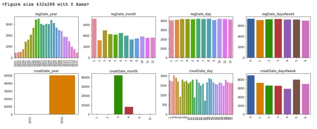
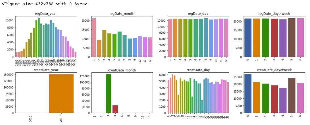
通過對于訓(xùn)練集和測試集的時(shí)間特征可視化，我們可以發(fā)現(xiàn)其分布是近似的,所以時(shí)間方面不會造成切換數(shù)據(jù)所導(dǎo)致的分布不一致的問題，進(jìn)一步的，這里對于數(shù)據(jù)特征和標(biāo)簽繪制箱型圖來判斷標(biāo)簽關(guān)于特征的分布差異性。

plt.figure()
plt.figure(figsize=(16, 6))
i = 1
for f in date_features:
    for col in ['year', 'month', 'day', 'dayofweek']:
        plt.subplot(2, 4, i)
        i += 1
        fig = sns.boxplot(x=Train_data[f + '_' + col], y=Train_data['price'])
        for item in fig.get_xticklabels():
            item.set_rotation(90)
        plt.title(f + '_' + col)
plt.tight_layout()
plt.show()

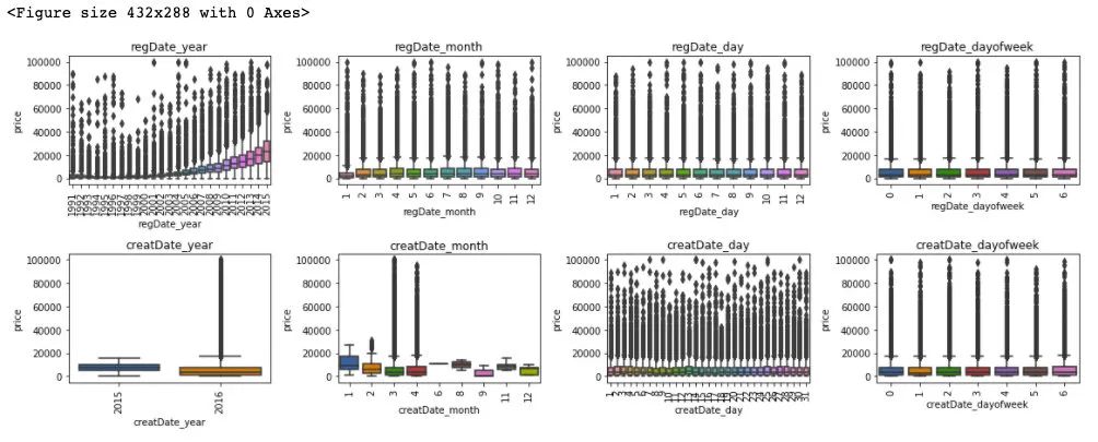
## 更新數(shù)據(jù)特征
date_features = ['regDate_year', 'regDate_month', 'regDate_day', 'regDate_dayofweek', 'creatDate_month', 'creatDate_day', 'creatDate_dayofweek']

可以發(fā)現(xiàn)，時(shí)間特征和價(jià)格的相關(guān)性來說，隨著 regDate_year 的時(shí)間越久遠(yuǎn)，其價(jià)格越低，然后 creatDate_month 特征和價(jià)格變化也有較大波動，但這通過前面的樣本統(tǒng)計(jì)量來看，是由于相對于3，4月份，剩余月份的樣本量較少的緣故。所以從時(shí)間特征中我們可以提前 regDate_year 作為模型預(yù)測的一個(gè)重要特征。

類別特征處理：

對于類別類型的特征，首先這里第一步進(jìn)行類別數(shù)量統(tǒng)計(jì)

from scipy.stats import mode

def sta_cate(df,cols):
    sta_df = pd.DataFrame(columns = ['column','nunique','miss_rate','most_value','most_value_counts','max_value_counts_rate'])
    for col in cols:
        count = df[col].count()
        nunique = df[col].nunique()
        miss_rate = (df.shape[0] - count) / df.shape[0]
        most_value = df[col].value_counts().index[0]
        most_value_counts = df[col].value_counts().values[0]
        max_value_counts_rate = most_value_counts / df.shape[0]
        
        sta_df = sta_df.append({'column':col,'nunique':nunique,'miss_rate':miss_rate,'most_value':most_value,
                                'most_value_counts':most_value_counts,'max_value_counts_rate':max_value_counts_rate},ignore_index=True)
    return sta_df
    

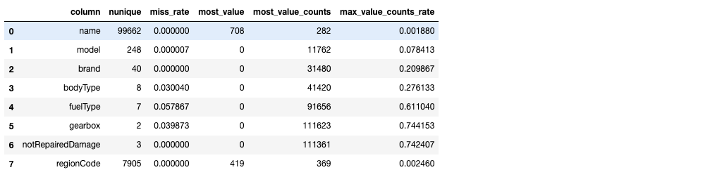
sta_cate(Train_data,categorical_features)

sta_cate(TestA_data,categorical_features)

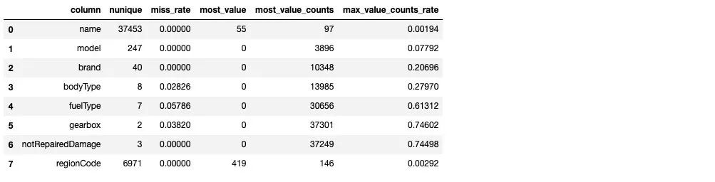
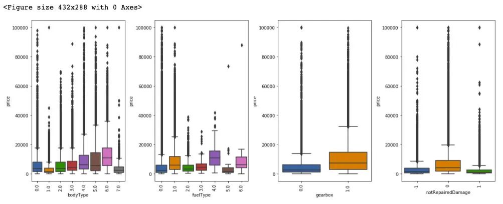
從上述樣本的統(tǒng)計(jì)情況來看,其中 name 特征和 regionCode 特征數(shù)量眾多，不適宜做類別編碼。model 特征需要做進(jìn)一步的考慮，這里我們先對于 剩余的類別特征做統(tǒng)計(jì)可視化：

plt.figure()
plt.figure(figsize=(16, 6))
i = 1
for col in ['bodyType', 'fuelType', 'gearbox', 'notRepairedDamage']:
    plt.subplot(1, 4, i)
    i += 1
    fig = sns.boxplot(x=Train_data[col], y=Train_data['price'])
    for item in fig.get_xticklabels():
        item.set_rotation(90)

plt.tight_layout()
plt.show()

from sklearn.preprocessing import LabelEncoder
from sklearn.preprocessing import OneHotEncoder

def cate_encoder(df,df_test,cols):
    le = LabelEncoder()
    ohe = OneHotEncoder(sparse=False,categories ='auto')
    
    for col in cols:
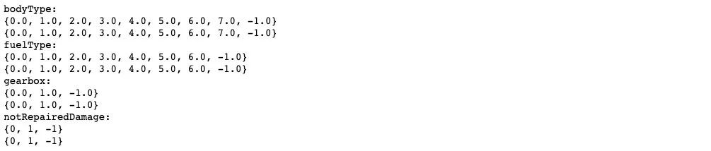
        print(col+':')
        print(set(df[col]))
        print(set(df_test[col]))
        
        le = le.fit(df[col])
        integer_encoded = le.transform(df[col])
        integer_encoded_test = le.transform(df_test[col])

        # binary encode
        integer_encoded = integer_encoded.reshape(len(integer_encoded), 1)
        integer_encoded_test = integer_encoded_test.reshape(len(integer_encoded_test), 1)
        ohe = ohe.fit(integer_encoded)
        
        onehot_encoded = ohe.transform(integer_encoded)
        onehot_encoded_df = pd.DataFrame(onehot_encoded)
        onehot_encoded_df.columns = list(map(lambda x:str(x)+'_'+col,onehot_encoded_df.columns.values))

        onehot_encoded_test = ohe.transform(integer_encoded_test)
        onehot_encoded_test_df = pd.DataFrame(onehot_encoded_test)
        onehot_encoded_test_df.columns = list(map(lambda x:str(x)+'_'+col,onehot_encoded_test_df.columns.values))
        
        df =  pd.concat([df,onehot_encoded_df], axis=1)
        df_test =  pd.concat([df_test,onehot_encoded_test_df], axis=1)
    
    return df,df_test

cate_cols = ['bodyType', 'fuelType', 'gearbox', 'notRepairedDamage']
Train_data[cate_cols] = Train_data[cate_cols].fillna(-1)
TestA_data[cate_cols] = TestA_data[cate_cols].fillna(-1)

Train_data,TestA_data = cate_encoder(Train_data,TestA_data,cate_cols)

## 對類別特征進(jìn)行 OneEncoder
# data = pd.get_dummies(data, columns=cate_cols)

Train_data

plt.figure(figsize=(15, 15))
i = 1
for col in numeric_features:
    plt.subplot(5, 4, i)
    i += 1
    sns.distplot(Train_data[col], label='train', color='r', hist=False)
    sns.distplot(TestA_data[col], label='test', color='b', hist=False)
plt.tight_layout()
plt.show()

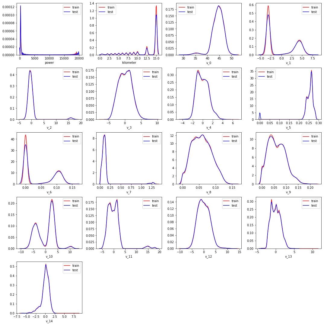
可以發(fā)現(xiàn)數(shù)值類型的特征分布在訓(xùn)練集和測試集上是近似的。

corr = Train_data[numeric_features+['price']].corr()
plt.figure(figsize=(20, 20))
sns.heatmap(abs(np.around(corr,2)), linewidths=0.1, annot=True,cmap=sns.cm.rocket_r)
plt.show()

從數(shù)值特征維度來看 v_0,v_3,v_8,v_12 和標(biāo)簽的線性相關(guān)性（皮爾遜相關(guān)系數(shù)）是較為相關(guān)的。

Step 4: 特征工程

1) 特征工程

# 訓(xùn)練集和測試集放在一起，方便構(gòu)造特征
Train_data['train']=1
TestA_data['train']=0

data = pd.concat([Train_data, TestA_data], ignore_index=True, sort=False)

一些特殊的特征生成：

data['used_time'] = (pd.to_datetime(data['creatDate'], format='%Y%m%d', errors='coerce') - 
                            pd.to_datetime(data['regDate'], format='%Y%m%d', errors='coerce')).dt.days

# 看一下空數(shù)據(jù)，有 15k 個(gè)樣本的時(shí)間是有問題的，我們可以選擇刪除，也可以選擇放著（不管或者作為一個(gè)單獨(dú)類別）。
# XGBoost 之類的決策樹，其本身就能處理缺失值，所以可以不用管；
data['used_time'].isnull().sum()

# Out：0

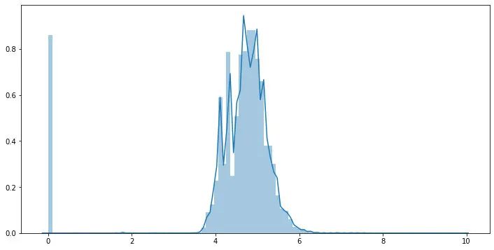
## 由于power 特征的分布特性，這里對于其進(jìn)行l(wèi)og變化
data['power'] = np.log1p(data['power'])

plt.figure(figsize=(12,6))
sns.distplot(data['power'].values ,bins=100)
plt.show()

# 計(jì)算某品牌的銷售統(tǒng)計(jì)量，這種特征不能細(xì)粒度的統(tǒng)計(jì)，防止發(fā)生信息過多的泄露
train_gb = Train_data.groupby("brand")
all_info = {}
for kind, kind_data in train_gb:
    info = {}
    kind_data = kind_data[kind_data['price'] > 0]
    info['brand_amount'] = len(kind_data)
    info['brand_price_max'] = kind_data.price.max()
    info['brand_price_median'] = kind_data.price.median()
    info['brand_price_min'] = kind_data.price.min()
    info['brand_price_sum'] = kind_data.price.sum()
    info['brand_price_std'] = kind_data.price.std()
    info['brand_price_average'] = round(kind_data.price.sum() / (len(kind_data) + 1), 2)
    all_info[kind] = info
brand_fe = pd.DataFrame(all_info).T.reset_index().rename(columns={"index": "brand"})
data = data.merge(brand_fe, how='left', on='brand')

統(tǒng)計(jì)特征生成：

統(tǒng)計(jì)特征這部分就有多種形式了，有多項(xiàng)式特征，類別和類別的交叉特征，類別和數(shù)值之間的交叉特征等

## 這部分就參考天才的代碼了
from scipy.stats import entropy

feat_cols = []

### count編碼
for f in tqdm(['regDate_year','model', 'brand', 'regionCode']):
    data[f + '_count'] = data[f].map(data[f].value_counts())
    feat_cols.append(f + '_count')

### 用數(shù)值特征對類別特征做統(tǒng)計(jì)刻畫，隨便挑了幾個(gè)跟price相關(guān)性最高的匿名特征
for f1 in tqdm(['model', 'brand', 'regionCode']):
    group = data.groupby(f1, as_index=False)
    for f2 in tqdm(['v_0', 'v_3', 'v_8', 'v_12']):
        feat = group[f2].agg({
            '{}_{}_max'.format(f1, f2): 'max', '{}_{}_min'.format(f1, f2): 'min',
            '{}_{}_median'.format(f1, f2): 'median', '{}_{}_mean'.format(f1, f2): 'mean',
            '{}_{}_std'.format(f1, f2): 'std', '{}_{}_mad'.format(f1, f2): 'mad'
        })
        data = data.merge(feat, on=f1, how='left')
        feat_list = list(feat)
        feat_list.remove(f1)
        feat_cols.extend(feat_list)


### 類別特征的二階交叉
for f_pair in tqdm([['model', 'brand'], ['model', 'regionCode'], ['brand', 'regionCode']]):
    ### 共現(xiàn)次數(shù)
    data['_'.join(f_pair) + '_count'] = data.groupby(f_pair)['SaleID'].transform('count')
    ### nunique、熵
    data = data.merge(data.groupby(f_pair[0], as_index=False)[f_pair[1]].agg({
        '{}_{}_nunique'.format(f_pair[0], f_pair[1]): 'nunique',
        '{}_{}_ent'.format(f_pair[0], f_pair[1]): lambda x: entropy(x.value_counts() / x.shape[0])
    }), on=f_pair[0], how='left')
    data = data.merge(data.groupby(f_pair[1], as_index=False)[f_pair[0]].agg({
        '{}_{}_nunique'.format(f_pair[1], f_pair[0]): 'nunique',
        '{}_{}_ent'.format(f_pair[1], f_pair[0]): lambda x: entropy(x.value_counts() / x.shape[0])
    }), on=f_pair[1], how='left')
    ### 比例偏好
    data['{}_in_{}_prop'.format(f_pair[0], f_pair[1])] = data['_'.join(f_pair) + '_count'] / data[f_pair[1] + '_count']
    data['{}_in_{}_prop'.format(f_pair[1], f_pair[0])] = data['_'.join(f_pair) + '_count'] / data[f_pair[0] + '_count']
    
    feat_cols.extend([
        '_'.join(f_pair) + '_count',
        '{}_{}_nunique'.format(f_pair[0], f_pair[1]), '{}_{}_ent'.format(f_pair[0], f_pair[1]),
        '{}_{}_nunique'.format(f_pair[1], f_pair[0]), '{}_{}_ent'.format(f_pair[1], f_pair[0]),
        '{}_in_{}_prop'.format(f_pair[0], f_pair[1]), '{}_in_{}_prop'.format(f_pair[1], f_pair[0])
    ])

data

train = data[data['train']==1]
test = data[data['train']==0]

categorical_cols = train.select_dtypes(include = 'object').columns
categorical_cols

# Out：Index([], dtype='object')

2) 構(gòu)建訓(xùn)練和測試樣本

## 選擇特征列
feature_cols = [col for col in data.columns if col not in ['SaleID','name','regDate','creatDate','price','model','brand',
            'regionCode','seller','bodyType','fuelType','offerType','train']]

feature_cols = [col for col in feature_cols if col not in date_features[1:]]

## 提前特征列，標(biāo)簽列構(gòu)造訓(xùn)練樣本和測試樣本
X_data = train[feature_cols]
Y_data = train['price']

X_test  = test[feature_cols]

print('X train shape:',X_data.shape)
print('X test shape:',X_test.shape)

### Out ### 
X train shape: (150000, 149)
X test shape: (50000, 149)

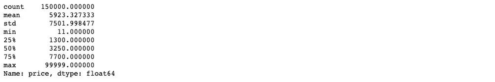
3) 統(tǒng)計(jì)標(biāo)簽的基本分布信息

Y_data.describe()

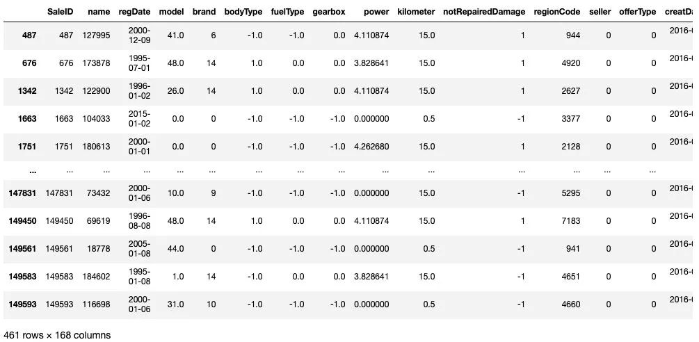
train[train['price']<1e2]

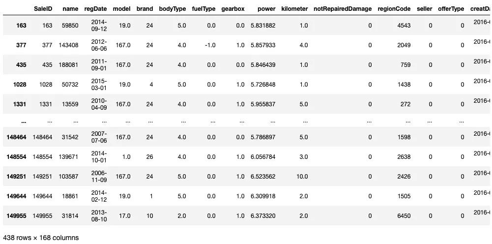
train[train['price']>5e4]

## 繪制標(biāo)簽的統(tǒng)計(jì)圖，查看標(biāo)簽分布
plt.figure(figsize=(12,6))
sns.distplot(Y_data,bins=100)
plt.show()

plt.figure(figsize=(12,6))
Y_data.plot.box()
plt.show()

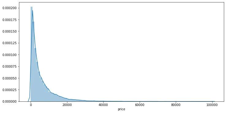
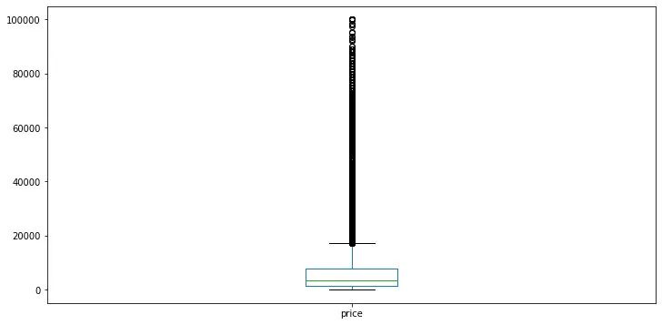
可以發(fā)現(xiàn)標(biāo)簽是非正態(tài)分布的，這里對于標(biāo)簽進(jìn)行l(wèi)og變換

Y_data_log = np.log1p(Y_data)

## 繪制標(biāo)簽的統(tǒng)計(jì)圖，查看標(biāo)簽log分布
plt.figure(figsize=(12,6))
sns.distplot(Y_data_log,bins=100)
plt.show()

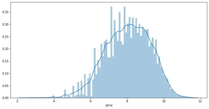
在實(shí)驗(yàn)中可以嘗試?yán)胠og后的標(biāo)簽訓(xùn)練再exp回去 和 直接用標(biāo)簽訓(xùn)練的效果進(jìn)行對比。

4) 缺省值用-1填補(bǔ)

X_data = X_data.fillna(-1)
X_test = X_test.fillna(-1)

Step 5: 模型構(gòu)建

這里分別舉例；1.利用交叉驗(yàn)證預(yù)測；2.模型混合預(yù)測。

1) 利用xgb進(jìn)行五折交叉驗(yàn)證查看模型的參數(shù)效果并預(yù)測

from sklearn.model_selection import KFold

def cv_predict(model,X_data,Y_data,X_test,sub):

    oof_trn = np.zeros(X_data.shape[0])
    oof_val = np.zeros(X_data.shape[0])

    ## 5折交叉驗(yàn)證方式
    kf = KFold(n_splits=5,shuffle=True,random_state=0)
    for idx, (trn_idx,val_idx) in enumerate(kf.split(X_data,Y_data)):
        print('--------------------- {} fold ---------------------'.format(idx))
        trn_x, trn_y = X_data.iloc[trn_idx].values, Y_data.iloc[trn_idx]
        val_x, val_y = X_data.iloc[val_idx].values, Y_data.iloc[val_idx]

        xgr.fit(trn_x,trn_y,eval_set=[(val_x, val_y)],eval_metric='mae',verbose=30,early_stopping_rounds=20,)

        oof_trn[trn_idx] = xgr.predict(trn_x)
        oof_val[val_idx] = xgr.predict(val_x)
        sub['price'] += xgr.predict(X_test.values) / kf.n_splits

        pred_trn_xgb=xgr.predict(trn_x)
        pred_val_xgb=xgr.predict(val_x)

        print('trn mae:', mean_absolute_error(trn_y, oof_trn[trn_idx]))
        print('val mae:', mean_absolute_error(val_y, oof_val[val_idx]))
    
    return model,oof_trn,oof_val,sub

## log標(biāo)簽預(yù)測
sub = test[['SaleID']].copy()
sub['price'] = 0

## xgb-Model
xgr = xgb.XGBRegressor(n_estimators=120, learning_rate=0.1, gamma=0, subsample=0.8,\
        colsample_bytree=0.9, max_depth=7) #,objective ='reg:squarederror'

model,oof_trn,oof_val,sub = cv_predict(xgr,X_data,Y_data_log,X_test,sub)

print('Train mae:',mean_absolute_error(Y_data_log,oof_trn))
print('Val mae:', mean_absolute_error(Y_data_log,oof_val))

print('Train mae trans:',mean_absolute_error(np.expm1(Y_data_log),np.expm1(oof_trn)))
print('Val mae trans', mean_absolute_error(np.expm1(Y_data_log),np.expm1(oof_val)))

## 原始標(biāo)簽預(yù)測
sub2 = test[['SaleID']].copy()
sub2['price'] = 0

oof_trn = np.zeros(train.shape[0])
oof_val = np.zeros(train.shape[0])

## xgb-Model
xgr = xgb.XGBRegressor(n_estimators=120, learning_rate=0.1, gamma=0, subsample=0.8,\
        colsample_bytree=0.9, max_depth=7) #,objective ='reg:squarederror'

model2,oof_trn,oof_val,sub2 = cv_predict(xgr,X_data,Y_data,X_test,sub2)

print('Train mae:',mean_squared_error(Y_data,oof_trn))
print('Val mae:', mean_squared_error(Y_data,oof_val))

2） 定義xgb和lgb模型函數(shù)，并對于lgb參數(shù)進(jìn)行網(wǎng)格化尋優(yōu)

def build_model_xgb(x_train,y_train):
    model = xgb.XGBRegressor(n_estimators=150, learning_rate=0.1, gamma=0, subsample=0.8,\
        colsample_bytree=0.9, max_depth=7) #, objective ='reg:squarederror'
    model.fit(x_train, y_train)
    return model

def build_model_lgb(x_train,y_train):
    estimator = lgb.LGBMRegressor(num_leaves=127,n_estimators = 150)
    param_grid = {
        'learning_rate': [0.01, 0.05, 0.1, 0.2],
    }
    gbm = GridSearchCV(estimator, param_grid)
    gbm.fit(x_train, y_train)
    return gbm

3）切分?jǐn)?shù)據(jù)集（Train,Val）進(jìn)行模型訓(xùn)練，評價(jià)和預(yù)測

## Split data with val
x_train,x_val,y_train,y_val = train_test_split(X_data,Y_data,test_size=0.3)

## 定義了一個(gè)統(tǒng)計(jì)函數(shù)，方便后續(xù)信息統(tǒng)計(jì)
def Sta_inf(data):
    print('_min',np.min(data))
    print('_max:',np.max(data))
    print('_mean',np.mean(data))
    print('_ptp',np.ptp(data))
    print('_std',np.std(data))
    print('_var',np.var(data))
    
print('Sta of label:')
Sta_inf(Y_data)

print('Train lgb...')
model_lgb = build_model_lgb(x_train,y_train)
val_lgb = model_lgb.predict(x_val)
MAE_lgb = mean_absolute_error(y_val,val_lgb)
print('MAE of val with lgb:',MAE_lgb)

print('Predict lgb...')
model_lgb_pre = build_model_lgb(X_data,Y_data)
subA_lgb = model_lgb_pre.predict(X_test)
print('Sta of Predict lgb:')
Sta_inf(subA_lgb)

print('Train xgb...')
model_xgb = build_model_xgb(x_train,y_train)
val_xgb = model_xgb.predict(x_val)
MAE_xgb = mean_absolute_error(y_val,val_xgb)
print('MAE of val with xgb:',MAE_xgb)

print('Predict xgb...')
model_xgb_pre = build_model_xgb(X_data,Y_data)
subA_xgb = model_xgb_pre.predict(X_test)
print('Sta of Predict xgb:')
Sta_inf(subA_xgb)

4）進(jìn)行兩模型的結(jié)果加權(quán)融合

## 這里我們采取了簡單的加權(quán)融合的方式
val_Weighted = (1-MAE_lgb/(MAE_xgb+MAE_lgb))*val_lgb+(1-MAE_xgb/(MAE_xgb+MAE_lgb))*val_xgb
val_Weighted[val_Weighted<10]=10 # 由于我們發(fā)現(xiàn)預(yù)測的最小值有負(fù)數(shù)，而真實(shí)情況下，price為負(fù)是不存在的，由此我們進(jìn)行對應(yīng)的后修正
print('MAE of val with Weighted ensemble:',mean_absolute_error(y_val,val_Weighted))

sub_Weighted = (1-MAE_lgb/(MAE_xgb+MAE_lgb))*subA_lgb+(1-MAE_xgb/(MAE_xgb+MAE_lgb))*subA_xgb
sub_Weighted[sub_Weighted<10]=10## 查看預(yù)測值的統(tǒng)計(jì),判斷和訓(xùn)練集是否接近
print('Sta of Predict lgb:')
Sta_inf(sub_Weighted)

5）輸出結(jié)果

sub3 = test[['SaleID']].copy()
sub3['price'] = sub_Weighted
sub3.to_csv('./sub_Weighted.csv',index=False)

sub3.head()

希望能幫助你完整實(shí)踐一場數(shù)據(jù)挖掘賽事。