一套完整的基于隨機(jī)森林的機(jī)器學(xué)習(xí)流程(特征選擇、交叉驗(yàn)證、模型評(píng)估))
機(jī)器學(xué)習(xí)實(shí)操(以隨機(jī)森林為例)
為了展示隨機(jī)森林的操作,我們用一套早期的前列腺癌和癌旁基因表達(dá)芯片數(shù)據(jù)集,包含102個(gè)樣品(50個(gè)正常,52個(gè)腫瘤),2個(gè)分組和9021個(gè)變量 (基因)。(https://file.biolab.si/biolab/supp/bi-cancer/projections/info/prostata.html)
數(shù)據(jù)格式和讀入數(shù)據(jù)
輸入數(shù)據(jù)為標(biāo)準(zhǔn)化之后的表達(dá)矩陣,基因在行,樣本在列。隨機(jī)森林對(duì)數(shù)值分布沒有假設(shè)。每個(gè)基因表達(dá)值用于分類時(shí)是基因內(nèi)部在不同樣品直接比較,只要是樣品之間標(biāo)準(zhǔn)化的數(shù)據(jù)即可,其他任何線性轉(zhuǎn)換如log2,scale等都沒有影響 (數(shù)據(jù)在:https://gitee.com/ct5869/shengxin-baodian/tree/master/machinelearning)。
樣品表達(dá)數(shù)據(jù):
prostat.expr.txt
樣品分組信息:
prostat.metadata.txt
expr_file <- "data/prostat.expr.symbol.txt"
metadata_file <- "data/prostat.metadata.txt"

# 每個(gè)基因表達(dá)值是內(nèi)部比較,只要是樣品之間標(biāo)準(zhǔn)化的數(shù)據(jù)即可,其它什么轉(zhuǎn)換都關(guān)系不大
# 機(jī)器學(xué)習(xí)時(shí),字符串還是默認(rèn)為因子類型的好
expr_mat <- read.table(expr_file, row.names = 1, header = T, sep="\t", stringsAsFactors =T)

# 處理異常的基因名字
rownames(expr_mat) <- make.names(rownames(expr_mat))

metadata <- read.table(metadata_file, row.names=1, header=T, sep="\t", stringsAsFactors =T)

dim(expr_mat)

## [1] 9021  102
基因表達(dá)表示例如下:
expr_mat[1:4,1:5]

##       normal_1 normal_2 normal_3 normal_4 normal_5
## AADAC      1.3       -1       -7       -4        5
## AAK1       0.4        0       10       11        8
## AAMP      -0.4       20       -7      -14       12
## AANAT    143.3       19      397      245      328
Metadata表示例如下
head(metadata)

##           class
## normal_1 normal
## normal_2 normal
## normal_3 normal
## normal_4 normal
## normal_5 normal
## normal_6 normal

table(metadata)

## metadata
## normal  tumor
##     50     52
樣品篩選和排序
對(duì)讀入的表達(dá)數(shù)據(jù)進(jìn)行轉(zhuǎn)置。通常我們是一行一個(gè)基因,一列一個(gè)樣品。在構(gòu)建模型時(shí),數(shù)據(jù)通常是反過來的,一列一個(gè)基因,一行一個(gè)樣品。每一列代表一個(gè)變量 (variable),每一行代表一個(gè)案例 (case)。這樣更方便提取每個(gè)變量,且易于把模型中的x,y放到一個(gè)矩陣中。
樣本表和表達(dá)表中的樣本順序對(duì)齊一致也是需要確保的一個(gè)操作。
# 表達(dá)數(shù)據(jù)轉(zhuǎn)置
# 習(xí)慣上我們是一行一個(gè)基因,一列一個(gè)樣品
# 做機(jī)器學(xué)習(xí)時(shí),大部分?jǐn)?shù)據(jù)都是反過來的,一列一個(gè)基因,一行一個(gè)樣品
# 每一列代表一個(gè)變量
expr_mat <- t(expr_mat)
expr_mat_sampleL <- rownames(expr_mat)
metadata_sampleL <- rownames(metadata)

common_sampleL <- intersect(expr_mat_sampleL, metadata_sampleL)

# 保證表達(dá)表樣品與METAdata樣品順序和數(shù)目完全一致
expr_mat <- expr_mat[common_sampleL,,drop=F]
metadata <- metadata[common_sampleL,,drop=F]
判斷是分類還是回歸
前面讀數(shù)據(jù)時(shí)已經(jīng)給定了參數(shù)stringsAsFactors =T,這一步可以忽略了。
如果group對(duì)應(yīng)的列為數(shù)字,轉(zhuǎn)換為數(shù)值型 - 做回歸
如果group對(duì)應(yīng)的列為分組,轉(zhuǎn)換為因子型 - 做分類
# R4.0之后默認(rèn)讀入的不是factor,需要做一個(gè)轉(zhuǎn)換
# devtools::install_github("Tong-Chen/ImageGP")
library(ImageGP)

# 此處的class根據(jù)需要修改
group = "class"

# 如果group對(duì)應(yīng)的列為數(shù)字,轉(zhuǎn)換為數(shù)值型 - 做回歸
# 如果group對(duì)應(yīng)的列為分組,轉(zhuǎn)換為因子型 - 做分類
if(numCheck(metadata[[group]])){
    if (!is.numeric(metadata[[group]])) {
      metadata[[group]] <- mixedToFloat(metadata[[group]])
    }
} else{
  metadata[[group]] <- as.factor(metadata[[group]])
}
隨機(jī)森林一般分析
library(randomForest)

# 查看參數(shù)是個(gè)好習(xí)慣
# 有了前面的基礎(chǔ)概述,再看每個(gè)參數(shù)的含義就明確了很多
# 也知道該怎么調(diào)了
# 每個(gè)人要解決的問題不同,通常不是別人用什么參數(shù),自己就跟著用什么參數(shù)
# 尤其是到下游分析時(shí)
# ?randomForest

# 查看源碼
# randomForest:::randomForest.default
加載包之后,直接分析一下,看到結(jié)果再調(diào)參。
# 設(shè)置隨機(jī)數(shù)種子,具體含義見 https://mp.weixin.qq.com/s/6plxo-E8qCdlzCgN8E90zg
set.seed(304)

# 直接使用默認(rèn)參數(shù)
rf <- randomForest(expr_mat, metadata[[group]])
查看下初步結(jié)果, 隨機(jī)森林類型判斷為分類,構(gòu)建了500棵樹,每次決策時(shí)從隨機(jī)選擇的94個(gè)基因中做最優(yōu)決策 (mtry),OOB估計(jì)的錯(cuò)誤率是9.8%,挺高的。
分類效果評(píng)估矩陣Confusion matrix,顯示normal組的分類錯(cuò)誤率為0.06,tumor組的分類錯(cuò)誤率為0.13。
rf

##
## Call:
##  randomForest(x = expr_mat, y = metadata[[group]])
##                Type of random forest: classification
##                      Number of trees: 500
## No. of variables tried at each split: 94
##
##         OOB estimate of  error rate: 9.8%
## Confusion matrix:
##        normal tumor class.error
## normal     47     3   0.0600000
## tumor       7    45   0.1346154
隨機(jī)森林標(biāo)準(zhǔn)操作流程 (適用于其他機(jī)器學(xué)習(xí)模型)
拆分訓(xùn)練集和測(cè)試集
library(caret)
seed <- 1
set.seed(seed)
train_index <- createDataPartition(metadata[[group]], p=0.75, list=F)
train_data <- expr_mat[train_index,]
train_data_group <- metadata[[group]][train_index]

test_data <- expr_mat[-train_index,]
test_data_group <- metadata[[group]][-train_index]

dim(train_data)

## [1]   77 9021

dim(test_data)

## [1]   25 9021
Boruta特征選擇鑒定關(guān)鍵分類變量
# install.packages("Boruta")
library(Boruta)
set.seed(1)

boruta <- Boruta(x=train_data, y=train_data_group, pValue=0.01, mcAdj=T,
       maxRuns=300)

boruta

## Boruta performed 299 iterations in 1.937513 mins.
##  46 attributes confirmed important: ADH5, AGR2, AKR1B1, ANGPT1,
## ANXA2.....ANXA2P1.....ANXA2P3 and 41 more;
##  8943 attributes confirmed unimportant: AADAC, AAK1, AAMP, AANAT, AARS
## and 8938 more;
##  32 tentative attributes left: ALDH2, ATP6V1G1, C16orf45, CDC42BPA,
## COL4A6 and 27 more;查看下變量重要性鑒定結(jié)果(實(shí)際上面的輸出中也已經(jīng)有體現(xiàn)了),54個(gè)重要的變量,36個(gè)可能重要的變量 (tentative variable, 重要性得分與最好的影子變量得分無統(tǒng)計(jì)差異),6,980個(gè)不重要的變量。
table(boruta$finalDecision)

##
## Tentative Confirmed  Rejected
##        32        46      8943
繪制鑒定出的變量的重要性。變量少了可以用默認(rèn)繪圖,變量多時(shí)繪制的圖看不清,需要自己整理數(shù)據(jù)繪圖。
定義一個(gè)函數(shù)提取每個(gè)變量對(duì)應(yīng)的重要性值。
library(dplyr)
boruta.imp <- function(x){
  imp <- reshape2::melt(x$ImpHistory, na.rm=T)[,-1]
  colnames(imp) <- c("Variable","Importance")
  imp <- imp[is.finite(imp$Importance),]

  variableGrp <- data.frame(Variable=names(x$finalDecision),
                            finalDecision=x$finalDecision)

  showGrp <- data.frame(Variable=c("shadowMax", "shadowMean", "shadowMin"),
                        finalDecision=c("shadowMax", "shadowMean", "shadowMin"))

  variableGrp <- rbind(variableGrp, showGrp)

  boruta.variable.imp <- merge(imp, variableGrp, all.x=T)

  sortedVariable <- boruta.variable.imp %>% group_by(Variable) %>%
    summarise(median=median(Importance)) %>% arrange(median)
  sortedVariable <- as.vector(sortedVariable$Variable)


  boruta.variable.imp$Variable <- factor(boruta.variable.imp$Variable, levels=sortedVariable)

  invisible(boruta.variable.imp)
}

boruta.variable.imp <- boruta.imp(boruta)

head(boruta.variable.imp)

##   Variable Importance finalDecision
## 1    AADAC          0      Rejected
## 2    AADAC          0      Rejected
## 3    AADAC          0      Rejected
## 4    AADAC          0      Rejected
## 5    AADAC          0      Rejected
## 6 AADAC 0 Rejected只繪制Confirmed變量。
library(ImageGP)

sp_boxplot(boruta.variable.imp, melted=T, xvariable = "Variable", yvariable = "Importance",
           legend_variable = "finalDecision", legend_variable_order = c("shadowMax", "shadowMean", "shadowMin", "Confirmed"),
           xtics_angle = 90)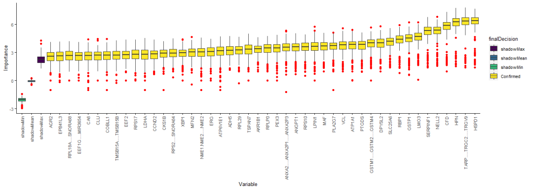
提取重要的變量和可能重要的變量
boruta.finalVarsWithTentative <- data.frame(Item=getSelectedAttributes(boruta, withTentative = T), Type="Boruta_with_tentative")看下這些變量的值的分布
caret::featurePlot(train_data[,boruta.finalVarsWithTentative$Item], train_data_group, plot="box")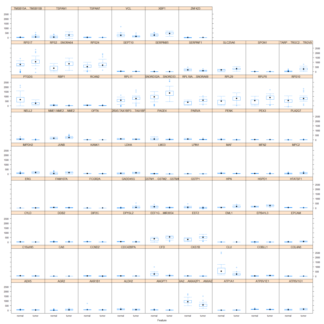
交叉驗(yàn)證選擇參數(shù)并擬合模型
定義一個(gè)函數(shù)生成一些列用來測(cè)試的mtry (一系列不大于總變量數(shù)的數(shù)值)。
generateTestVariableSet <- function(num_toal_variable){
  max_power <- ceiling(log10(num_toal_variable))
  tmp_subset <- c(unlist(sapply(1:max_power, function(x) (1:10)^x, simplify = F)), ceiling(max_power/3))
  #return(tmp_subset)
  base::unique(sort(tmp_subset[tmp_subset<num_toal_variable]))
}
# generateTestVariableSet(78)
選擇關(guān)鍵特征變量相關(guān)的數(shù)據(jù)
# 提取訓(xùn)練集的特征變量子集
boruta_train_data <- train_data[, boruta.finalVarsWithTentative$Item]
boruta_mtry <- generateTestVariableSet(ncol(boruta_train_data))
使用 Caret 進(jìn)行調(diào)參和建模
library(caret)
# Create model with default parameters
trControl <- trainControl(method="repeatedcv", number=10, repeats=5)

seed <- 1
set.seed(seed)
# 根據(jù)經(jīng)驗(yàn)或感覺設(shè)置一些待查詢的參數(shù)和參數(shù)值
tuneGrid <- expand.grid(mtry=boruta_mtry)

borutaConfirmed_rf_default <- train(x=boruta_train_data, y=train_data_group, method="rf",
                                    tuneGrid = tuneGrid, #
                                    metric="Accuracy", #metric='Kappa'
                                    trControl=trControl)
borutaConfirmed_rf_default

## Random Forest
##
## 77 samples
## 78 predictors
##  2 classes: 'normal', 'tumor'
##
## No pre-processing
## Resampling: Cross-Validated (10 fold, repeated 5 times)
## Summary of sample sizes: 71, 69, 69, 69, 69, 69, ...
## Resampling results across tuning parameters:
##
##   mtry  Accuracy   Kappa
##    1    0.9352381  0.8708771
##    2    0.9352381  0.8708771
##    3    0.9352381  0.8708771
##    4    0.9377381  0.8758771
##    5    0.9377381  0.8758771
##    6    0.9402381  0.8808771
##    7    0.9402381  0.8808771
##    8    0.9452381  0.8908771
##    9    0.9402381  0.8808771
##   10    0.9452381  0.8908771
##   16    0.9452381  0.8908771
##   25    0.9477381  0.8958771
##   36    0.9452381  0.8908771
##   49    0.9402381  0.8808771
##   64    0.9327381  0.8658771
##
## Accuracy was used to select the optimal model using the largest value.
## The final value used for the model was mtry = 25.
可視化不同參數(shù)的準(zhǔn)確性分布
plot(borutaConfirmed_rf_default)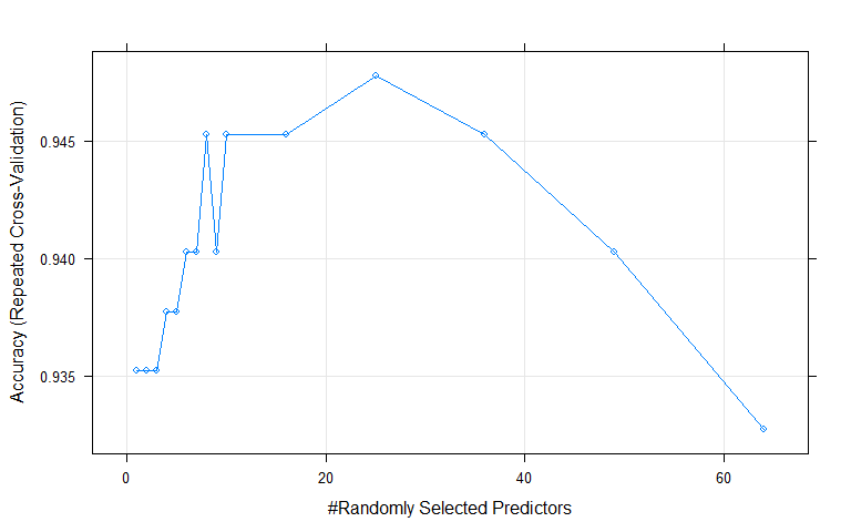 可視化Top20重要的變量
dotPlot(varImp(borutaConfirmed_rf_default))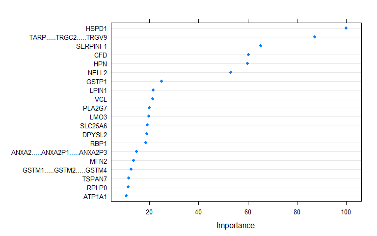
提取最終選擇的模型,并繪制 ROC 曲線評(píng)估模型
borutaConfirmed_rf_default_finalmodel <- borutaConfirmed_rf_default$finalModel先自評(píng),評(píng)估模型對(duì)訓(xùn)練集的分類效果
采用訓(xùn)練數(shù)據(jù)集評(píng)估構(gòu)建的模型,Accuracy=1; Kappa=1,非常完美。
模型的預(yù)測(cè)顯著性P-Value [Acc > NIR] : 2.2e-16。其中NIR是No Information Rate,其計(jì)算方式為數(shù)據(jù)集中最大的類包含的數(shù)據(jù)占總數(shù)據(jù)集的比例。如某套數(shù)據(jù)中,分組A有80個(gè)樣品,分組B有20個(gè)樣品,我們只要猜A,正確率就會(huì)有80%,這就是NIR。如果基于這套數(shù)據(jù)構(gòu)建的模型準(zhǔn)確率也是80%,那么這個(gè)看上去準(zhǔn)確率較高的模型也沒有意義。confusionMatrix使用binom.test函數(shù)檢驗(yàn)?zāi)P偷臏?zhǔn)確性Accuracy是否顯著優(yōu)于NIR,若P-value<0.05,則表示模型預(yù)測(cè)準(zhǔn)確率顯著高于隨便猜測(cè)。
# 獲得模型結(jié)果評(píng)估矩陣(`confusion matrix`)

predictions_train <- predict(borutaConfirmed_rf_default_finalmodel, newdata=train_data)
confusionMatrix(predictions_train, train_data_group)

## Confusion Matrix and Statistics
##
##           Reference
## Prediction normal tumor
##     normal     38     0
##     tumor       0    39
##
##                Accuracy : 1
##                  95% CI : (0.9532, 1)
##     No Information Rate : 0.5065
##     P-Value [Acc > NIR] : < 2.2e-16
##
##                   Kappa : 1
##
##  Mcnemar's Test P-Value : NA
##
##             Sensitivity : 1.0000
##             Specificity : 1.0000
##          Pos Pred Value : 1.0000
##          Neg Pred Value : 1.0000
##              Prevalence : 0.4935
##          Detection Rate : 0.4935
##    Detection Prevalence : 0.4935
##       Balanced Accuracy : 1.0000
##
##        'Positive' Class : normal
##
盲評(píng),評(píng)估模型應(yīng)用于測(cè)試集時(shí)的效果
繪制ROC曲線,計(jì)算模型整體的AUC值,并選擇最佳模型。
# 繪制ROC曲線

prediction_prob <- predict(borutaConfirmed_rf_default_finalmodel, newdata=test_data, type="prob")
library(pROC)
roc_curve <- roc(test_data_group, prediction_prob[,1])

roc_curve

##
## Call:
## roc.default(response = test_data_group, predictor = prediction_prob[,     1])
##
## Data: prediction_prob[, 1] in 12 controls (test_data_group normal) > 13 cases (test_data_group tumor).
## Area under the curve: 0.9872

# roc <- roc(test_data_group, factor(predictions, ordered=T))
# plot(roc)
基于默認(rèn)閾值的盲評(píng)
基于默認(rèn)閾值繪制混淆矩陣并評(píng)估模型預(yù)測(cè)準(zhǔn)確度顯著性,結(jié)果顯著P-Value [Acc > NIR]<0.05。
# 獲得模型結(jié)果評(píng)估矩陣(`confusion matrix`)

predictions <- predict(borutaConfirmed_rf_default_finalmodel, newdata=test_data)
confusionMatrix(predictions, test_data_group)

## Confusion Matrix and Statistics
##
##           Reference
## Prediction normal tumor
##     normal     12     2
##     tumor       0    11
##
##                Accuracy : 0.92
##                  95% CI : (0.7397, 0.9902)
##     No Information Rate : 0.52
##     P-Value [Acc > NIR] : 2.222e-05
##
##                   Kappa : 0.8408
##
##  Mcnemar's Test P-Value : 0.4795
##
##             Sensitivity : 1.0000
##             Specificity : 0.8462
##          Pos Pred Value : 0.8571
##          Neg Pred Value : 1.0000
##              Prevalence : 0.4800
##          Detection Rate : 0.4800
##    Detection Prevalence : 0.5600
##       Balanced Accuracy : 0.9231
##
##        'Positive' Class : normal
##
選擇模型分類最佳閾值再盲評(píng)
youden:max(sensitivities?+?r?×?specificities)
closest.topleft:min((1???sensitivities)2?+?r?×?(1???specificities)2)
r是加權(quán)系數(shù),默認(rèn)是1,其計(jì)算方式為r?=?(1???prevalenc**e)/(cos**t?*?prevalenc**e).
best.weights控制加權(quán)方式:(cost, prevalence)默認(rèn)是(1,0.5),據(jù)此算出的r為1。
cost: 假陰性率占假陽性率的比例,容忍更高的假陽性率還是假陰性率
prevalence: 關(guān)注的類中的個(gè)體所占的比例 (
n.cases/(n.controls+n.cases)).
best_thresh <- data.frame(coords(roc=roc_curve, x = "best", input="threshold",
                                 transpose = F, best.method = "youden"))

best_thresh$best <- apply(best_thresh, 1, function (x)
  paste0('threshold: ', x[1], ' (', round(1-x[2],3), ", ", round(x[3],3), ")"))

best_thresh

##   threshold specificity sensitivity                        best
## 1     0.672   0.9166667           1 threshold: 0.672 (0.083, 1)
準(zhǔn)備數(shù)據(jù)繪制ROC曲線
library(ggrepel)
ROC_data <- data.frame(FPR = 1- roc_curve$specificities, TPR=roc_curve$sensitivities)
ROC_data <- ROC_data[with(ROC_data, order(FPR,TPR)),]
p <- ggplot(data=ROC_data, mapping=aes(x=FPR, y=TPR)) +
geom_step(color="red", size=1, direction = "vh") +
geom_segment(aes(x=0, xend=1, y=0, yend=1)) + theme_classic() +
xlab("False positive rate") +
ylab("True positive rate") + coord_fixed(1) + xlim(0,1) + ylim(0,1) +
annotate('text', x=0.5, y=0.25, label=paste('AUC=', round(roc_curve$auc,2))) +
geom_point(data=best_thresh, mapping=aes(x=1-specificity, y=sensitivity), color='blue', size=2) +
geom_text_repel(data=best_thresh, mapping=aes(x=1.05-specificity, y=sensitivity ,label=best))
p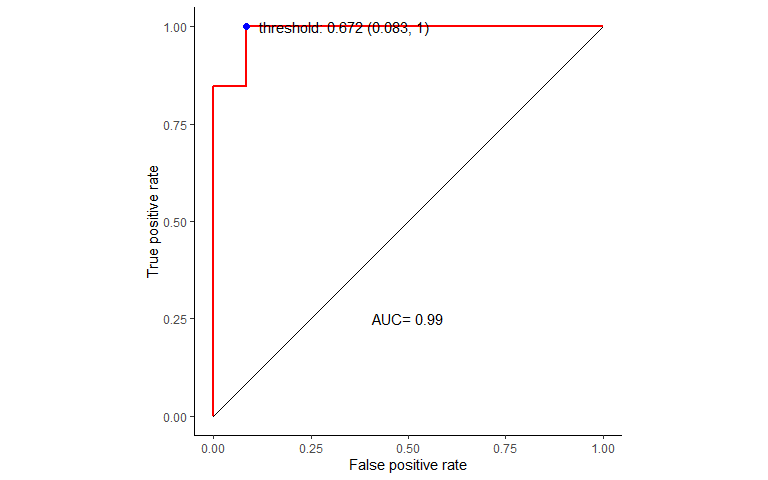 基于選定的最優(yōu)閾值制作混淆矩陣并評(píng)估模型預(yù)測(cè)準(zhǔn)確度顯著性,結(jié)果顯著
P-Value [Acc > NIR]<0.05。
predict_result <- data.frame(Predict_status=c(T,F), Predict_class=colnames(prediction_prob))

head(predict_result)

##   Predict_status Predict_class
## 1           TRUE        normal
## 2          FALSE         tumor

predictions2 <- plyr::join(data.frame(Predict_status=prediction_prob[,1] > best_thresh[1,1]), predict_result)

predictions2 <- as.factor(predictions2$Predict_class)

confusionMatrix(predictions2, test_data_group)

## Confusion Matrix and Statistics
##
##           Reference
## Prediction normal tumor
##     normal     11     0
##     tumor       1    13
##
##                Accuracy : 0.96
##                  95% CI : (0.7965, 0.999)
##     No Information Rate : 0.52
##     P-Value [Acc > NIR] : 1.913e-06
##
##                   Kappa : 0.9196
##
##  Mcnemar's Test P-Value : 1
##
##             Sensitivity : 0.9167
##             Specificity : 1.0000
##          Pos Pred Value : 1.0000
##          Neg Pred Value : 0.9286
##              Prevalence : 0.4800
##          Detection Rate : 0.4400
##    Detection Prevalence : 0.4400
##       Balanced Accuracy : 0.9583
##
##        'Positive' Class : normal
##
機(jī)器學(xué)習(xí)系列教程
從隨機(jī)森林開始,一步步理解決策樹、隨機(jī)森林、ROC/AUC、數(shù)據(jù)集、交叉驗(yàn)證的概念和實(shí)踐。
文字能說清的用文字、圖片能展示的用、描述不清的用公式、公式還不清楚的寫個(gè)簡(jiǎn)單代碼,一步步理清各個(gè)環(huán)節(jié)和概念。
再到成熟代碼應(yīng)用、模型調(diào)參、模型比較、模型評(píng)估,學(xué)習(xí)整個(gè)機(jī)器學(xué)習(xí)需要用到的知識(shí)和技能。
往期精品(點(diǎn)擊圖片直達(dá)文字對(duì)應(yīng)教程)
|
|
|
|
|
|
|
|
|
|
|
|
|
|
|
|
|
|
|
|
|
|
|
|
|
|
|


后臺(tái)回復(fù)“生信寶典福利第一波”或點(diǎn)擊閱讀原文獲取教程合集