機器學習第20篇 - 基于Boruta選擇的特征變量構(gòu)建隨機森林

前面機器學習第18篇 - Boruta特征變量篩選（2）已經(jīng)完成了特征變量篩選，下面看下基于篩選的特征變量構(gòu)建的模型準確性怎樣？

定義一個函數(shù)生成一些列用來測試的mtry (一系列不大于總變量數(shù)的數(shù)值)。

generateTestVariableSet <- function(num_toal_variable){
  max_power <- ceiling(log10(num_toal_variable))
  tmp_subset <- unique(unlist(sapply(1:max_power, function(x) (1:10)^x, simplify = F)))
  sort(tmp_subset[tmp_subset}

選擇關(guān)鍵特征變量相關(guān)的數(shù)據(jù)

# withTentative=F: 不包含tentative變量
boruta.confirmed <- getSelectedAttributes(boruta, withTentative = F)

# 提取訓練集的特征變量子集
boruta_train_data <- train_data[, boruta.confirmed]
boruta_mtry <- generateTestVariableSet(length(boruta.confirmed))

使用 Caret 進行調(diào)參和建模

library(caret)
# Create model with default parameters
trControl <- trainControl(method="repeatedcv", number=10, repeats=5)

# train model
if(file.exists('rda/borutaConfirmed_rf_default.rda')){
   borutaConfirmed_rf_default <- readRDS("rda/borutaConfirmed_rf_default.rda")
} else {
  # 設(shè)置隨機數(shù)種子，使得結(jié)果可重復
  seed <- 1
  set.seed(seed)
  # 根據(jù)經(jīng)驗或感覺設(shè)置一些待查詢的參數(shù)和參數(shù)值
  tuneGrid <- expand.grid(mtry=boruta_mtry)

  borutaConfirmed_rf_default <- train(x=boruta_train_data, y=train_data_group, method="rf", 
                     tuneGrid = tuneGrid, # 
                     metric="Accuracy", #metric='Kappa'
                     trControl=trControl)
  saveRDS(borutaConfirmed_rf_default, "rda/borutaConfirmed_rf_default.rda")
}
print(borutaConfirmed_rf_default)

在使用Boruta選擇的特征變量后，模型的準確性和Kappa值都提升了很多。

## Random Forest 
## 
## 59 samples
## 56 predictors
##  2 classes: 'DLBCL', 'FL' 
## 
## No pre-processing
## Resampling: Cross-Validated (10 fold, repeated 5 times) 
## Summary of sample sizes: 53, 54, 53, 54, 53, 52, ... 
## Resampling results across tuning parameters:
## 
##   mtry  Accuracy   Kappa    
##    1    0.9862857  0.9565868
##    2    0.9632381  0.8898836
##    3    0.9519048  0.8413122
##    4    0.9519048  0.8413122
##    5    0.9519048  0.8413122
##    6    0.9519048  0.8413122
##    7    0.9552381  0.8498836
##    8    0.9519048  0.8413122
##    9    0.9547619  0.8473992
##   10    0.9519048  0.8413122
##   16    0.9479048  0.8361174
##   25    0.9519048  0.8413122
##   36    0.9450476  0.8282044
##   49    0.9421905  0.8199691
## 
## Accuracy was used to select the optimal model using the largest value.
## The final value used for the model was mtry = 1.

提取最終選擇的模型，并繪制 ROC 曲線。

borutaConfirmed_rf_default_finalmodel <- borutaConfirmed_rf_default$finalModel

采用訓練數(shù)據(jù)集評估構(gòu)建的模型，Accuracy=1; Kappa=1，訓練的非常完美。

模型的預測顯著性P-Value [Acc > NIR] : 3.044e-08。其中NIR是No Information Rate，其計算方式為數(shù)據(jù)集中最大的類包含的數(shù)據(jù)占總數(shù)據(jù)集的比例。如某套數(shù)據(jù)中，分組A有80個樣品，分組B有20個樣品，我們只要猜A，正確率就會有80%，這就是NIR。如果基于這套數(shù)據(jù)構(gòu)建的模型準確率也是80%，那么這個看上去準確率較高的模型也沒有意義。

confusionMatrix使用binom.test函數(shù)檢驗模型的準確性Accuracy是否顯著優(yōu)于NIR，若P-value<0.05，則表示模型預測準確率顯著高于隨便猜測。

# 獲得模型結(jié)果評估矩陣(`confusion matrix`)

predictions_train <- predict(borutaConfirmed_rf_default_finalmodel, newdata=train_data)
confusionMatrix(predictions_train, train_data_group)

## Confusion Matrix and Statistics
## 
##           Reference
## Prediction DLBCL FL
##      DLBCL    44  0
##      FL        0 15
##                                      
##                Accuracy : 1          
##                  95% CI : (0.9394, 1)
##     No Information Rate : 0.7458     
##     P-Value [Acc > NIR] : 3.044e-08  
##                                      
##                   Kappa : 1          
##                                      
##  Mcnemar's Test P-Value : NA         
##                                      
##             Sensitivity : 1.0000     
##             Specificity : 1.0000     
##          Pos Pred Value : 1.0000     
##          Neg Pred Value : 1.0000     
##              Prevalence : 0.7458     
##          Detection Rate : 0.7458     
##    Detection Prevalence : 0.7458     
##       Balanced Accuracy : 1.0000     
##                                      
##        'Positive' Class : DLBCL      
##

繪制ROC曲線，計算模型整體的AUC值，并選擇最佳閾值。

# 繪制ROC曲線

prediction_prob <- predict(borutaConfirmed_rf_default_finalmodel, newdata=test_data, type="prob")
library(pROC)
roc_curve <- roc(test_data_group, prediction_prob[,1])
#roc <- roc(test_data_group, factor(predictions, ordered=T))

roc_curve

## 
## Call:
## roc.default(response = test_data_group, predictor = prediction_prob[,     1])
## 
## Data: prediction_prob[, 1] in 14 controls (test_data_group DLBCL) > 4 cases (test_data_group FL).
## Area under the curve: 0.9821

選擇最佳閾值，在控制假陽性率的基礎(chǔ)上獲得高的敏感性

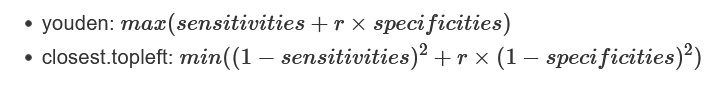
r是加權(quán)系數(shù)，默認是1，其計算方式為r=(1−prevalence)/(cost∗prevalence)" role="presentation">r=(1?prevalence)/(cost?prevalence).

best.weights控制加權(quán)方式：(cost, prevalence)默認是(1, 0.5)，據(jù)此算出的r為1。

• cost: 假陰性率占假陽性率的比例，容忍更高的假陽性率還是假陰性率

• prevalence: 關(guān)注的類中的個體所占的比例 (n.cases/(n.controls+n.cases)).

best_thresh <- data.frame(coords(roc=roc_curve, x = "best", input="threshold", 
                                 transpose = F, best.method = "youden"))
best_thresh

##   threshold specificity sensitivity
## 1     0.736   0.9285714           1

準備數(shù)據(jù)繪制ROC曲線

library(ggrepel)
ROC_data <- data.frame(FPR = 1- roc_curve$specificities, TPR=roc_curve$sensitivities)
ROC_data <- ROC_data[with(ROC_data, order(FPR,TPR)),]

best_thresh$best <- apply(best_thresh, 1, function (x) 
  paste0('threshold: ', x[1], ' (', round(1-x[2],3), ", ", round(x[3],3), ")"))

p <- ggplot(data=ROC_data, mapping=aes(x=FPR, y=TPR)) +
  geom_step(color="red", size=1, direction = "vh") +
  geom_segment(aes(x=0, xend=1, y=0, yend=1))  + theme_classic() + 
  xlab("False positive rate") + 
  ylab("True positive rate") + coord_fixed(1) + xlim(0,1) + ylim(0,1) +
  annotate('text', x=0.5, y=0.25, label=paste('AUC=', round(roc$auc,2))) +
  geom_point(data=best_thresh, mapping=aes(x=1-specificity, y=sensitivity), color='blue', size=2) + 
  geom_text_repel(data=best_thresh, mapping=aes(x=1.05-specificity, y=sensitivity ,label=best))
p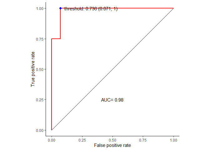

基于默認閾值繪制混淆矩陣并評估模型預測準確度顯著性，結(jié)果不顯著P-Value [Acc > NIR]>0.05。

# 獲得模型結(jié)果評估矩陣(`confusion matrix`)

predictions <- predict(borutaConfirmed_rf_default_finalmodel, newdata=test_data)
confusionMatrix(predictions, test_data_group)

## Confusion Matrix and Statistics
## 
##           Reference
## Prediction DLBCL FL
##      DLBCL    14  1
##      FL        0  3
##                                           
##                Accuracy : 0.9444          
##                  95% CI : (0.7271, 0.9986)
##     No Information Rate : 0.7778          
##     P-Value [Acc > NIR] : 0.06665         
##                                           
##                   Kappa : 0.8235          
##                                           
##  Mcnemar's Test P-Value : 1.00000         
##                                           
##             Sensitivity : 1.0000          
##             Specificity : 0.7500          
##          Pos Pred Value : 0.9333          
##          Neg Pred Value : 1.0000          
##              Prevalence : 0.7778          
##          Detection Rate : 0.7778          
##    Detection Prevalence : 0.8333          
##       Balanced Accuracy : 0.8750          
##                                           
##        'Positive' Class : DLBCL           
##

基于選定的最優(yōu)閾值制作混淆矩陣并評估模型預測準確度顯著性,結(jié)果還是不顯著 P-Value [Acc > NIR]>0.05。

predict_result <- data.frame(Predict_status=c(T,F), Predict_class=colnames(prediction_prob))

head(predict_result)

##   Predict_status Predict_class
## 1           TRUE         DLBCL
## 2          FALSE            FL

predictions2 <- plyr::join(data.frame(Predict_status=prediction_prob[,1] > best_thresh[1,1]), predict_result)

predictions2 <- as.factor(predictions2$Predict_class)

confusionMatrix(predictions2, test_data_group)

## Confusion Matrix and Statistics
## 
##           Reference
## Prediction DLBCL FL
##      DLBCL    13  0
##      FL        1  4
##                                           
##                Accuracy : 0.9444          
##                  95% CI : (0.7271, 0.9986)
##     No Information Rate : 0.7778          
##     P-Value [Acc > NIR] : 0.06665         
##                                           
##                   Kappa : 0.8525          
##                                           
##  Mcnemar's Test P-Value : 1.00000         
##                                           
##             Sensitivity : 0.9286          
##             Specificity : 1.0000          
##          Pos Pred Value : 1.0000          
##          Neg Pred Value : 0.8000          
##              Prevalence : 0.7778          
##          Detection Rate : 0.7222          
##    Detection Prevalence : 0.7222          
##       Balanced Accuracy : 0.9643          
##                                           
##        'Positive' Class : DLBCL           
##

篩選完特征變量后，模型的準確性和Kappa值都提高了很多。但統(tǒng)計檢驗卻還是提示不顯著，這可能是數(shù)據(jù)不平衡的問題，我們后續(xù)繼續(xù)優(yōu)化。

機器學習系列教程

從隨機森林開始，一步步理解決策樹、隨機森林、ROC/AUC、數(shù)據(jù)集、交叉驗證的概念和實踐。

文字能說清的用文字、圖片能展示的用、描述不清的用公式、公式還不清楚的寫個簡單代碼，一步步理清各個環(huán)節(jié)和概念。

再到成熟代碼應用、模型調(diào)參、模型比較、模型評估，學習整個機器學習需要用到的知識和技能。

1. 機器學習算法 - 隨機森林之決策樹初探（1）

2. 機器學習算法-隨機森林之決策樹R 代碼從頭暴力實現(xiàn)（2）

3. 機器學習算法-隨機森林之決策樹R 代碼從頭暴力實現(xiàn)（3）

4. 機器學習算法-隨機森林之理論概述

5. 隨機森林拖了這么久，終于到實戰(zhàn)了。先分享很多套用于機器學習的多種癌癥表達數(shù)據(jù)集 https://file.biolab.si/biolab/supp/bi-cancer/projections/。

6. 機器學習算法-隨機森林初探（1）
   

7. 機器學習 模型評估指標 - ROC曲線和AUC值

8. 機器學習 - 訓練集、驗證集、測試集

9. 機器學習 - 隨機森林手動10 折交叉驗證

10. 一個函數(shù)統(tǒng)一238個機器學習R包，這也太贊了吧

11. 基于Caret和RandomForest包進行隨機森林分析的一般步驟 （1）

12. Caret模型訓練和調(diào)參更多參數(shù)解讀(2)

13. 機器學習相關(guān)書籍分享

14. 基于Caret進行隨機森林隨機調(diào)參的4種方式

15. 送你一個在線機器學習網(wǎng)站，真香！

16. UCI機器學習數(shù)據(jù)集

17. 機器學習第17篇 - 特征變量篩選（1）

18. 機器學習第18篇 - 基于隨機森林的Boruta特征變量篩選（2）

19. 機器學習系列補充：數(shù)據(jù)集準備和更正YSX包